CNModel Tutorial
Trey V. Wenger (c) April 2025
Here we demonstrate the basic features of the CNModel model. The CNModel models the hyperfine spectral structure of \({\rm CN}\) and \(^{13}{\rm CN}\) including non-LTE effects. Please review the bayes_spec documentation and tutorials for a more thorough description of the steps outlined in this tutorial: https://bayes-spec.readthedocs.io/en/stable/index.html
[1]:
# General imports
import os
import pickle
import time

import matplotlib.pyplot as plt
import arviz as az
import pandas as pd
import numpy as np
import pymc as pm

print("arviz version:", az.__version__)

print("pymc version:", pm.__version__)

import bayes_spec
print("bayes_spec version:", bayes_spec.__version__)

import bayes_cn_hfs
print("bayes_cn_hfs version:", bayes_cn_hfs.__version__)

# Notebook configuration
pd.options.display.max_rows = None
arviz version: 0.22.0dev
pymc version: 5.21.1
bayes_spec version: 1.7.8
bayes_cn_hfs version: 2.0.0-staging+0.g7afe3a8.dirty
supplement_mol_data
Here we model the hyperfine structure of CN emission. We use the helper function supplement_mol_data to download the molecular data for this molecule.
[2]:
from bayes_cn_hfs import supplement_mol_data

mol_data_12CN, mol_weight_12CN = supplement_mol_data("CN")
print(mol_data_12CN.keys())
print("transition frequency (MHz):", mol_data_12CN['freq'])
print("Einstein A coefficient (s-1):", mol_data_12CN['Aul'])
print("Upper state degrees of freedom:", mol_data_12CN['degu'])
print("Lower state energy level (erg)", mol_data_12CN['El'])
print("Upper state energy level (erg)", mol_data_12CN['Eu'])
print("Relative intensities", mol_data_12CN['relative_int'])
print("Partition function terms:", mol_data_12CN["log10_Q_terms"])
print("Upper state quantum numbers:", mol_data_12CN["Qu"])
print("lower states quantum numbers", mol_data_12CN["Ql"])
print("state info", mol_data_12CN["states"])
dict_keys(['freq', 'Aul', 'degu', 'El', 'Eu', 'relative_int', 'log10_Q_terms', 'Qu', 'Ql', 'states', 'state_u_idx', 'state_l_idx', 'Gu', 'Gl'])
transition frequency (MHz): [113123.3687 113144.19   113170.535  113191.325  113488.142  113490.985
 113499.643  113508.934  113520.4215]
Einstein A coefficient (s-1): [1.26969616e-06 1.03939111e-05 5.07869910e-06 6.59525390e-06
 6.64784064e-06 1.17706070e-05 1.04919208e-05 5.12459350e-06
 1.28243028e-06]
Upper state degrees of freedom: [2 2 4 4 4 6 2 4 2]
Lower state energy level (erg) [1.3905121e-19 0.0000000e+00 1.3905121e-19 0.0000000e+00 1.3905121e-19
 0.0000000e+00 1.3905121e-19 0.0000000e+00 0.0000000e+00]
Upper state energy level (erg) [7.49702428e-16 7.49701340e-16 7.50014955e-16 7.50013660e-16
 7.52119441e-16 7.51999228e-16 7.52195648e-16 7.52118159e-16
 7.52194276e-16]
Relative intensities [0.01204699 0.09860036 0.09633376 0.1250773  0.12574146 0.33394774
 0.09921527 0.09691221 0.01212491]
Partition function terms: [0.40307694 0.97433601]
Upper state quantum numbers: [np.str_('1 0 1 1'), np.str_('1 0 1 1'), np.str_('1 0 1 2'), np.str_('1 0 1 2'), np.str_('1 0 2 2'), np.str_('1 0 2 3'), np.str_('1 0 2 1'), np.str_('1 0 2 2'), np.str_('1 0 2 1')]
lower states quantum numbers [np.str_('0 0 1 1'), np.str_('0 0 1 2'), np.str_('0 0 1 1'), np.str_('0 0 1 2'), np.str_('0 0 1 1'), np.str_('0 0 1 2'), np.str_('0 0 1 1'), np.str_('0 0 1 2'), np.str_('0 0 1 2')]
state info {'state': [np.str_('0 0 1 1'), np.str_('0 0 1 2'), np.str_('1 0 1 1'), np.str_('1 0 1 2'), np.str_('1 0 2 1'), np.str_('1 0 2 2'), np.str_('1 0 2 3')], 'deg': array([2, 4, 2, 4, 2, 4, 6]), 'E': array([1.00714381e-03, 0.00000000e+00, 5.43007258e+00, 5.43233621e+00,
       5.44813090e+00, 5.44757894e+00, 5.44670824e+00])}
Simulating Data
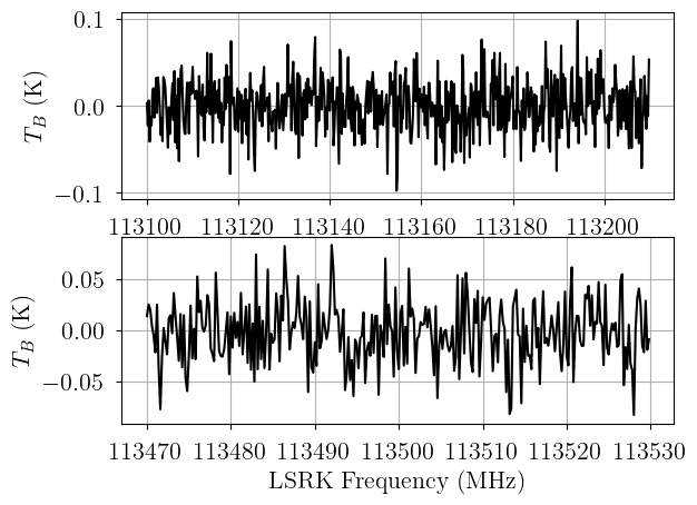
To test the model, we must simulate some data. We can do this with CNModel, but we must pack a “dummy” data structure first.
[3]:
from bayes_spec import SpecData

# spectral axis definition
freq_axis_1 = np.arange(113100.0, 113210.0, 0.2) # MHz
freq_axis_2 = np.arange(113470.0, 113530.0, 0.2) # MHz

# data noise can either be a scalar (assumed constant noise across the spectrum)
# or an array of the same length as the data
noise = 0.03 # K

# brightness data. In this case, we just throw in some random data for now
# since we are only doing this in order to simulate some actual data.
brightness_data_1 = noise * np.random.randn(len(freq_axis_1)) # K
brightness_data_2 = noise * np.random.randn(len(freq_axis_2)) # K

# CNModel datasets can be named anything, here we name them "12CN-1" and "12CN-2"
obs_1 = SpecData(
    freq_axis_1,
    brightness_data_1,
    noise,
    xlabel=r"LSRK Frequency (MHz)",
    ylabel=r"$T_B$ (K)",
)
obs_2 = SpecData(
    freq_axis_2,
    brightness_data_2,
    noise,
    xlabel=r"LSRK Frequency (MHz)",
    ylabel=r"$T_B$ (K)",
)
dummy_data = {"12CN-1": obs_1, "12CN-2": obs_2}

# Plot the simulated data
fig, axes = plt.subplots(2)
axes[0].plot(dummy_data["12CN-1"].spectral, dummy_data["12CN-1"].brightness, "k-")
axes[0].set_ylabel(dummy_data["12CN-1"].ylabel)
axes[1].plot(dummy_data["12CN-2"].spectral, dummy_data["12CN-2"].brightness, "k-")
axes[1].set_xlabel(dummy_data["12CN-2"].xlabel)
_ = axes[1].set_ylabel(dummy_data["12CN-2"].ylabel)
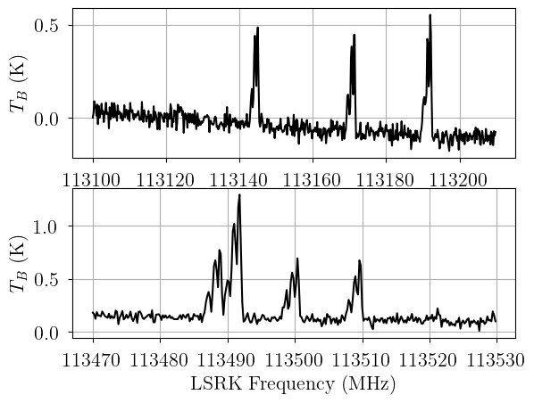
Now that we have a dummy data format, we can generate a simulated observation by evaluating the model for a given set of parameters.
[4]:
from bayes_cn_hfs.cn_model import CNModel

# Initialize and define the model
n_clouds = 3 # number of cloud components
baseline_degree = 2 # polynomial baseline degree
model = CNModel(
    dummy_data,
    molecule="CN", # molecule (either "CN" or "13CN")
    mol_data=mol_data_12CN, # molecular data
    bg_temp = 2.7, # assumed background temperature (K)
    Beff = 1.0, # beam efficiency
    Feff = 1.0, # forward efficiency
    n_clouds=n_clouds,
    baseline_degree=baseline_degree,
    seed=1234,
    verbose=True
)
model.add_priors(
    prior_log10_N = [13.5, 1.0], # mean and width of log10 total column density prior (cm-2)
    prior_log10_Tkin = [1.0, 0.5], # mean and width of log10 kinetic temperature prior (K)
    prior_velocity = [0.0, 5.0], # mean and width of velocity prior (km/s)
    prior_fwhm_nonthermal = 1.0, # width of non-thermal broadening prior (km/s)
    prior_fwhm_L = None, # assume Gaussian line profile
    prior_rms = None, # do not infer spectral rms
    prior_baseline_coeffs = None, # use default baseline priors
    assume_LTE = True, # assume kinetic temperature = excitation temperature
    prior_log10_Tex = None, # ignored for this LTE model
    assume_CTEX = True, # assume CTEX
    prior_log10_LTE_precision = None, # ignored for this LTE model
    fix_log10_Tkin = None, # do not fix the kinetic temperature
    clip_weights = 1.0e-9, # clip statistical weights between [clip_weights, 1-clip_weights]
    clip_tau = -10.0, # clip optical depths below to prevent masers
    ordered = False, # do not assume optically-thin
)
model.add_likelihood()

sim_params = {
    "log10_N": [13.8, 13.9, 14.0],
    "log10_Tkin": [0.65, 0.6, 0.5],
    "fwhm_nonthermal": [1.0, 1.25, 1.5],
    "velocity": [-2.0, 0.0, 2.5],
    "fwhm_L": 0.0,
    "baseline_12CN-1_norm": [-2.0, -5.0, 8.0],
    "baseline_12CN-2_norm": [4.0, -2.0, 5.0],
}

# add derived quantities to sim_params
for key in model.cloud_deterministics:
    if key not in sim_params.keys():
        sim_params[key] = model.model[key].eval(sim_params, on_unused_input="ignore")

# Evaluate and save simulated observations
sim_obs1 = model.model["12CN-1"].eval(sim_params, on_unused_input="ignore")
sim_obs2 = model.model["12CN-2"].eval(sim_params, on_unused_input="ignore")

# Plot the simulated data
fig, axes = plt.subplots(2)
axes[0].plot(dummy_data["12CN-1"].spectral, sim_obs1, "k-")
axes[0].set_ylabel(dummy_data["12CN-1"].ylabel)
axes[1].plot(dummy_data["12CN-2"].spectral, sim_obs2, "k-")
axes[1].set_xlabel(dummy_data["12CN-2"].xlabel)
_ = axes[1].set_ylabel(dummy_data["12CN-2"].ylabel)
[5]:
sim_params
[5]:
{'log10_N': [13.8, 13.9, 14.0],
 'log10_Tkin': [0.65, 0.6, 0.5],
 'fwhm_nonthermal': [1.0, 1.25, 1.5],
 'velocity': [-2.0, 0.0, 2.5],
 'fwhm_L': 0.0,
 'baseline_12CN-1_norm': [-2.0, -5.0, 8.0],
 'baseline_12CN-2_norm': [4.0, -2.0, 5.0],
 'fwhm_thermal': array([0.08867757, 0.08371703, 0.07461288]),
 'fwhm': array([1.00392416, 1.25280028, 1.50185455]),
 'log10_Tex_ul': array([0.65, 0.6 , 0.5 ]),
 'LTE_weights': array([[0.17659718, 0.353274  , 0.05237634, 0.10469961, 0.05216502,
         0.10434294, 0.15654492],
        [0.18885791, 0.37781138, 0.04829246, 0.09653001, 0.04807389,
         0.09616112, 0.14427323],
        [0.21685988, 0.43385792, 0.0389559 , 0.07785605, 0.03873407,
         0.07748167, 0.11625451]]),
 'Tex': array([[4.46683592, 3.98107171, 3.16227766],
        [4.46683592, 3.98107171, 3.16227766],
        [4.46683592, 3.98107171, 3.16227766],
        [4.46683592, 3.98107171, 3.16227766],
        [4.46683592, 3.98107171, 3.16227766],
        [4.46683592, 3.98107171, 3.16227766],
        [4.46683592, 3.98107171, 3.16227766],
        [4.46683592, 3.98107171, 3.16227766],
        [4.46683592, 3.98107171, 3.16227766]]),
 'tau': array([[0.02780937, 0.03961643, 0.06312223],
        [0.22764058, 0.32429648, 0.51673788],
        [0.2223333 , 0.31672379, 0.5046276 ],
        [0.28871089, 0.41128963, 0.65532851],
        [0.28981529, 0.41280405, 0.65753902],
        [0.76986139, 1.09659601, 1.7468342 ],
        [0.22866526, 0.32570236, 0.51879336],
        [0.22339835, 0.31820796, 0.50688522],
        [0.02794853, 0.03980962, 0.06341362]]),
 'tau_total': array([2.30618295, 3.28504631, 5.23328165]),
 'TR': array([[2.28910526, 1.86520154, 1.1888105 ],
        [2.28879859, 1.86491585, 1.18857141],
        [2.28841062, 1.86455441, 1.18826896],
        [2.2881045 , 1.86426923, 1.18803032],
        [2.28373743, 1.86020143, 1.1846276 ],
        [2.28369563, 1.8601625 , 1.18459504],
        [2.28356835, 1.86004396, 1.18449591],
        [2.28343176, 1.85991675, 1.18438954],
        [2.28326289, 1.85975948, 1.18425803]])}
[6]:
# Now we pack the simulated spectrum into a new SpecData instance
obs_1 = SpecData(
    freq_axis_1,
    sim_obs1,
    noise,
    xlabel=r"LSRK Frequency (MHz)",
    ylabel=r"$T_B$ (K)",
)
obs_2 = SpecData(
    freq_axis_2,
    sim_obs2,
    noise,
    xlabel=r"LSRK Frequency (MHz)",
    ylabel=r"$T_B$ (K)",
)
data = {"12CN-1": obs_1, "12CN-2": obs_2}
Model Definition
Finally, with our model definition and (simulated) data in hand, we can explore the capabilities of CNModel. Here we create a new model with the simulated data. We assume LTE.
[7]:
# Initialize and define the model
model = CNModel(
    data,
    molecule="CN", # molecule (either "CN" or "13CN")
    mol_data=mol_data_12CN, # molecular data
    bg_temp = 2.7, # assumed background temperature (K)
    Beff = 1.0, # beam efficiency
    Feff = 1.0, # forward efficiency
    n_clouds=n_clouds,
    baseline_degree=baseline_degree,
    seed=1234,
    verbose=True
)
model.add_priors(
    prior_log10_N = [13.5, 1.0], # mean and width of log10 total column density prior (cm-2)
    prior_log10_Tkin = [1.0, 0.5], # mean and width of log10 kinetic temperature prior (K)
    prior_velocity = [0.0, 5.0], # mean and width of velocity prior (km/s)
    prior_fwhm_nonthermal = 1.0, # width of non-thermal broadening prior (km/s)
    prior_fwhm_L = None, # assume Gaussian line profile
    prior_rms = None, # do not infer spectral rms
    prior_baseline_coeffs = None, # use default baseline priors
    assume_LTE = True, # assume kinetic temperature = excitation temperature
    prior_log10_Tex = None, # ignored for this LTE model
    assume_CTEX = True, # assume CTEX
    prior_log10_LTE_precision = None, # ignored for this LTE model
    fix_log10_Tkin = None, # do not fix the kinetic temperature
    clip_weights = 1.0e-9, # clip statistical weights between [clip_weights, 1-clip_weights]
    clip_tau = -10.0, # clip optical depths below to prevent masers
    ordered = False, # do not assume optically-thin
)
model.add_likelihood()
[8]:
# Plot model graph
model.graph().render('cn_model', format='png')
model.graph()
[8]:

[9]:
# model string representation
print(model.model.str_repr())
baseline_12CN-1_norm ~ Normal(0, <constant>)
baseline_12CN-2_norm ~ Normal(0, <constant>)
       velocity_norm ~ Normal(0, 1)
     log10_Tkin_norm ~ Normal(0, 1)
fwhm_nonthermal_norm ~ HalfNormal(0, 1)
        log10_N_norm ~ Normal(0, 1)
            velocity ~ Deterministic(f(velocity_norm))
          log10_Tkin ~ Deterministic(f(log10_Tkin_norm))
        fwhm_thermal ~ Deterministic(f(log10_Tkin_norm))
     fwhm_nonthermal ~ Deterministic(f(fwhm_nonthermal_norm))
                fwhm ~ Deterministic(f(fwhm_nonthermal_norm, log10_Tkin_norm))
             log10_N ~ Deterministic(f(log10_N_norm))
        log10_Tex_ul ~ Deterministic(f(log10_Tkin_norm))
         LTE_weights ~ Deterministic(f(log10_Tkin_norm))
                 Tex ~ Deterministic(f(log10_Tkin_norm))
                 tau ~ Deterministic(f(log10_N_norm, log10_Tkin_norm))
           tau_total ~ Deterministic(f(log10_N_norm, log10_Tkin_norm))
                  TR ~ Deterministic(f(log10_Tkin_norm))
              12CN-1 ~ Normal(f(baseline_12CN-1_norm, log10_Tkin_norm, velocity_norm, log10_N_norm, fwhm_nonthermal_norm), <constant>)
              12CN-2 ~ Normal(f(baseline_12CN-2_norm, log10_Tkin_norm, velocity_norm, log10_N_norm, fwhm_nonthermal_norm), <constant>)
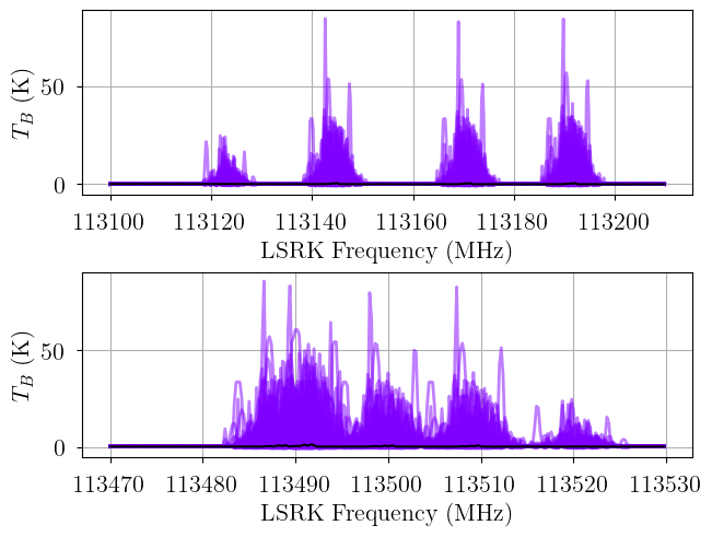
We check that our prior distributions are reasonable by drawing prior predictive checks. Each colored line is a simulated “observation” with parameters drawn from the prior distributions. You should check that these simulated observations at least somewhat overlap your actual observation (black line).
[10]:
from bayes_spec.plots import plot_predictive

# prior predictive check
prior = model.sample_prior_predictive(
    samples=1000,  # prior predictive samples
)
_ = plot_predictive(model.data, prior.prior_predictive)
Sampling: [12CN-1, 12CN-2, baseline_12CN-1_norm, baseline_12CN-2_norm, fwhm_nonthermal_norm, log10_N_norm, log10_Tkin_norm, velocity_norm]
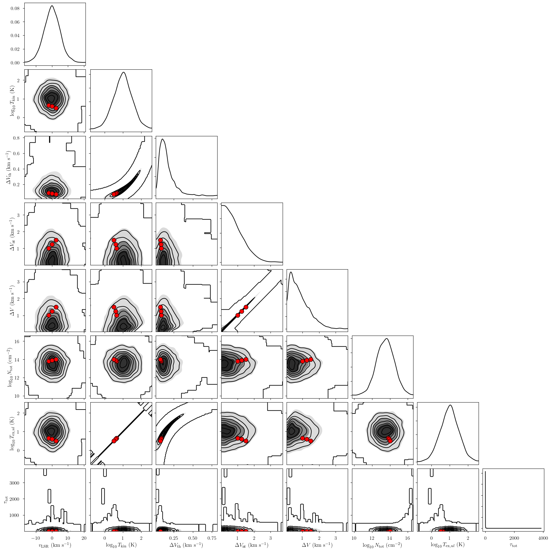
We can also generate a pair plot to inspect the prior distributions and their effect on deterministic quantities. The model has several attributes to access the various free parameters (freeRVs) and deterministic quantities (deterministics). Here we show the pair plot for the deterministic quantities derived from our prior distributions. The three red points correspond to the simulation parameters (“truths”) for our three clouds.
[11]:
from bayes_spec.plots import plot_pair

# available parameter attributes:
print("baseline_freeRVs", model.baseline_freeRVs)
print("baseline_deterministics", model.baseline_deterministics)
print("cloud_freeRVs", model.cloud_freeRVs)
print("cloud_deterministics", model.cloud_deterministics)
print("hyper_freeRVs", model.hyper_freeRVs)
print("hyper_deterministics", model.hyper_deterministics)

# ignore transition and state dependent parameters
var_names = [
    param for param in model.cloud_deterministics
    if not set(model.model.named_vars_to_dims[param]).intersection(set(["transition", "state"]))
]
_ = plot_pair(
    prior.prior, # samples
    var_names, # var_names to plot
    labeller=model.labeller, # label manager
    kind="kde", # plot type
    reference_values=sim_params, # truths
)
baseline_freeRVs ['baseline_12CN-1_norm', 'baseline_12CN-2_norm']
baseline_deterministics []
cloud_freeRVs ['velocity_norm', 'log10_Tkin_norm', 'fwhm_nonthermal_norm', 'log10_N_norm']
cloud_deterministics ['velocity', 'log10_Tkin', 'fwhm_thermal', 'fwhm_nonthermal', 'fwhm', 'log10_N', 'log10_Tex_ul', 'LTE_weights', 'Tex', 'tau', 'tau_total', 'TR']
hyper_freeRVs []
hyper_deterministics []
Variational Inference
We can approximate the posterior distribution using variational inference.
[12]:
start = time.time()
model.fit(
    n = 100_000, # maximum number of VI iterations
    draws = 1_000, # number of posterior samples
    rel_tolerance = 0.05, # VI relative convergence threshold
    abs_tolerance = 0.05, # VI absolute convergence threshold
    learning_rate = 0.01, # VI learning rate
)
end = time.time()
print(f"Runtime: {(end-start)/60.0:.2f} minutes")
Convergence achieved at 8800
Interrupted at 8,799 [8%]: Average Loss = 1,173.3
Runtime: 0.29 minutes
[13]:
posterior = model.sample_posterior_predictive(
    thin=100, # keep one in {thin} posterior samples
)
_ = plot_predictive(model.data, posterior.posterior_predictive)
Sampling: [12CN-1, 12CN-2]
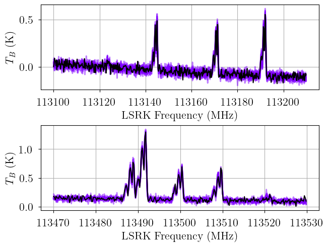
Posterior Sampling: MCMC
We can sample from the posterior distribution using MCMC.
[14]:
start = time.time()
init_kwargs = {
    "rel_tolerance": 0.05,
    "abs_tolerance": 0.05,
    "learning_rate": 0.01,
}
model.sample(
    init = "advi+adapt_diag", # initialization strategy
    tune = 1000, # tuning samples
    draws = 1000, # posterior samples
    chains = 8, # number of independent chains
    cores = 8, # number of parallel chains
    init_kwargs = init_kwargs, # VI initialization arguments
    nuts_kwargs = {"target_accept": 0.8}, # NUTS arguments
)
end = time.time()
print(f"Runtime: {(end-start)/60.0:.2f} minutes")
Initializing NUTS using custom advi+adapt_diag strategy
Convergence achieved at 8800
Interrupted at 8,799 [8%]: Average Loss = 1,173.3
Multiprocess sampling (8 chains in 8 jobs)
NUTS: [baseline_12CN-1_norm, baseline_12CN-2_norm, velocity_norm, log10_Tkin_norm, fwhm_nonthermal_norm, log10_N_norm]
Sampling 8 chains for 1_000 tune and 1_000 draw iterations (8_000 + 8_000 draws total) took 54 seconds.
Adding log-likelihood to trace
Runtime: 1.30 minutes
[15]:
model.solve(kl_div_threshold=0.1)
GMM converged to unique solution
[16]:
print("solutions:", model.solutions)

pm.summary(model.trace.solution_0)
solutions: [0]
[16]:
| mean | sd | hdi_3% | hdi_97% | mcse_mean | mcse_sd | ess_bulk | ess_tail | r_hat | |
|---|---|---|---|---|---|---|---|---|---|
| baseline_12CN-1_norm[0] | -0.214 | 0.053 | -0.316 | -0.117 | 0.001 | 0.001 | 9051.0 | 6947.0 | 1.0 |
| baseline_12CN-1_norm[1] | -4.779 | 0.141 | -5.034 | -4.508 | 0.001 | 0.002 | 15012.0 | 6024.0 | 1.0 |
| baseline_12CN-1_norm[2] | 2.186 | 0.793 | 0.684 | 3.617 | 0.008 | 0.008 | 9344.0 | 6753.0 | 1.0 |
| baseline_12CN-2_norm[0] | -0.316 | 0.071 | -0.447 | -0.183 | 0.001 | 0.001 | 10084.0 | 6640.0 | 1.0 |
| baseline_12CN-2_norm[1] | -1.990 | 0.202 | -2.362 | -1.599 | 0.002 | 0.002 | 13096.0 | 6114.0 | 1.0 |
| baseline_12CN-2_norm[2] | 0.433 | 0.888 | -1.242 | 2.045 | 0.008 | 0.010 | 11282.0 | 6694.0 | 1.0 |
| velocity_norm[0] | 0.004 | 0.003 | -0.002 | 0.009 | 0.000 | 0.000 | 10185.0 | 6176.0 | 1.0 |
| velocity_norm[1] | -0.400 | 0.002 | -0.404 | -0.397 | 0.000 | 0.000 | 10409.0 | 6524.0 | 1.0 |
| velocity_norm[2] | 0.510 | 0.007 | 0.496 | 0.523 | 0.000 | 0.000 | 10767.0 | 6333.0 | 1.0 |
| log10_Tkin_norm[0] | -0.799 | 0.013 | -0.823 | -0.776 | 0.000 | 0.000 | 7311.0 | 6343.0 | 1.0 |
| log10_Tkin_norm[1] | -0.697 | 0.016 | -0.725 | -0.666 | 0.000 | 0.000 | 6276.0 | 5382.0 | 1.0 |
| log10_Tkin_norm[2] | -0.985 | 0.015 | -1.012 | -0.959 | 0.000 | 0.000 | 5838.0 | 5259.0 | 1.0 |
| log10_N_norm[0] | 0.409 | 0.026 | 0.362 | 0.459 | 0.000 | 0.000 | 7280.0 | 6375.0 | 1.0 |
| log10_N_norm[1] | 0.297 | 0.022 | 0.256 | 0.339 | 0.000 | 0.000 | 6354.0 | 5683.0 | 1.0 |
| log10_N_norm[2] | 0.425 | 0.064 | 0.303 | 0.543 | 0.001 | 0.001 | 6089.0 | 5224.0 | 1.0 |
| fwhm_nonthermal_norm[0] | 1.291 | 0.040 | 1.217 | 1.365 | 0.000 | 0.000 | 7479.0 | 6463.0 | 1.0 |
| fwhm_nonthermal_norm[1] | 1.007 | 0.026 | 0.959 | 1.055 | 0.000 | 0.000 | 8232.0 | 6164.0 | 1.0 |
| fwhm_nonthermal_norm[2] | 1.499 | 0.089 | 1.330 | 1.657 | 0.001 | 0.001 | 8609.0 | 6598.0 | 1.0 |
| velocity[0] | 0.019 | 0.015 | -0.009 | 0.046 | 0.000 | 0.000 | 10185.0 | 6176.0 | 1.0 |
| velocity[1] | -2.002 | 0.010 | -2.022 | -1.983 | 0.000 | 0.000 | 10409.0 | 6524.0 | 1.0 |
| velocity[2] | 2.549 | 0.036 | 2.480 | 2.617 | 0.000 | 0.000 | 10767.0 | 6333.0 | 1.0 |
| log10_Tkin[0] | 0.601 | 0.006 | 0.588 | 0.612 | 0.000 | 0.000 | 7311.0 | 6343.0 | 1.0 |
| log10_Tkin[1] | 0.652 | 0.008 | 0.637 | 0.667 | 0.000 | 0.000 | 6276.0 | 5382.0 | 1.0 |
| log10_Tkin[2] | 0.507 | 0.007 | 0.494 | 0.521 | 0.000 | 0.000 | 5838.0 | 5259.0 | 1.0 |
| fwhm_thermal[0] | 0.084 | 0.001 | 0.083 | 0.085 | 0.000 | 0.000 | 7311.0 | 6343.0 | 1.0 |
| fwhm_thermal[1] | 0.089 | 0.001 | 0.087 | 0.090 | 0.000 | 0.000 | 6276.0 | 5382.0 | 1.0 |
| fwhm_thermal[2] | 0.075 | 0.001 | 0.074 | 0.076 | 0.000 | 0.000 | 5838.0 | 5259.0 | 1.0 |
| fwhm_nonthermal[0] | 1.291 | 0.040 | 1.217 | 1.365 | 0.000 | 0.000 | 7479.0 | 6463.0 | 1.0 |
| fwhm_nonthermal[1] | 1.007 | 0.026 | 0.959 | 1.055 | 0.000 | 0.000 | 8232.0 | 6164.0 | 1.0 |
| fwhm_nonthermal[2] | 1.499 | 0.089 | 1.330 | 1.657 | 0.001 | 0.001 | 8609.0 | 6598.0 | 1.0 |
| fwhm[0] | 1.294 | 0.040 | 1.220 | 1.368 | 0.000 | 0.000 | 7477.0 | 6463.0 | 1.0 |
| fwhm[1] | 1.011 | 0.026 | 0.963 | 1.058 | 0.000 | 0.000 | 8222.0 | 6189.0 | 1.0 |
| fwhm[2] | 1.501 | 0.089 | 1.332 | 1.659 | 0.001 | 0.001 | 8608.0 | 6598.0 | 1.0 |
| log10_N[0] | 13.909 | 0.026 | 13.862 | 13.959 | 0.000 | 0.000 | 7280.0 | 6375.0 | 1.0 |
| log10_N[1] | 13.797 | 0.022 | 13.756 | 13.839 | 0.000 | 0.000 | 6354.0 | 5683.0 | 1.0 |
| log10_N[2] | 13.925 | 0.064 | 13.803 | 14.043 | 0.001 | 0.001 | 6089.0 | 5224.0 | 1.0 |
| log10_Tex_ul[0] | 0.601 | 0.006 | 0.588 | 0.612 | 0.000 | 0.000 | 7311.0 | 6343.0 | 1.0 |
| log10_Tex_ul[1] | 0.652 | 0.008 | 0.637 | 0.667 | 0.000 | 0.000 | 6276.0 | 5382.0 | 1.0 |
| log10_Tex_ul[2] | 0.507 | 0.007 | 0.494 | 0.521 | 0.000 | 0.000 | 5838.0 | 5259.0 | 1.0 |
| LTE_weights[0, 0 0 1 1] | 0.189 | 0.002 | 0.186 | 0.192 | 0.000 | 0.000 | 7311.0 | 6343.0 | 1.0 |
| LTE_weights[0, 0 0 1 2] | 0.377 | 0.003 | 0.371 | 0.383 | 0.000 | 0.000 | 7311.0 | 6343.0 | 1.0 |
| LTE_weights[0, 1 0 1 1] | 0.048 | 0.001 | 0.047 | 0.049 | 0.000 | 0.000 | 7311.0 | 6343.0 | 1.0 |
| LTE_weights[0, 1 0 1 2] | 0.097 | 0.001 | 0.095 | 0.099 | 0.000 | 0.000 | 7311.0 | 6343.0 | 1.0 |
| LTE_weights[0, 1 0 2 1] | 0.048 | 0.001 | 0.047 | 0.049 | 0.000 | 0.000 | 7311.0 | 6343.0 | 1.0 |
| LTE_weights[0, 1 0 2 2] | 0.096 | 0.001 | 0.094 | 0.098 | 0.000 | 0.000 | 7311.0 | 6343.0 | 1.0 |
| LTE_weights[0, 1 0 2 3] | 0.144 | 0.002 | 0.141 | 0.148 | 0.000 | 0.000 | 7311.0 | 6343.0 | 1.0 |
| LTE_weights[1, 0 0 1 1] | 0.176 | 0.002 | 0.173 | 0.180 | 0.000 | 0.000 | 6276.0 | 5382.0 | 1.0 |
| LTE_weights[1, 0 0 1 2] | 0.353 | 0.004 | 0.346 | 0.359 | 0.000 | 0.000 | 6276.0 | 5382.0 | 1.0 |
| LTE_weights[1, 1 0 1 1] | 0.053 | 0.001 | 0.051 | 0.054 | 0.000 | 0.000 | 6276.0 | 5382.0 | 1.0 |
| LTE_weights[1, 1 0 1 2] | 0.105 | 0.001 | 0.103 | 0.107 | 0.000 | 0.000 | 6276.0 | 5382.0 | 1.0 |
| LTE_weights[1, 1 0 2 1] | 0.052 | 0.001 | 0.051 | 0.053 | 0.000 | 0.000 | 6276.0 | 5382.0 | 1.0 |
| LTE_weights[1, 1 0 2 2] | 0.105 | 0.001 | 0.102 | 0.107 | 0.000 | 0.000 | 6276.0 | 5382.0 | 1.0 |
| LTE_weights[1, 1 0 2 3] | 0.157 | 0.002 | 0.154 | 0.160 | 0.000 | 0.000 | 6276.0 | 5382.0 | 1.0 |
| LTE_weights[2, 0 0 1 1] | 0.215 | 0.002 | 0.210 | 0.218 | 0.000 | 0.000 | 5838.0 | 5259.0 | 1.0 |
| LTE_weights[2, 0 0 1 2] | 0.429 | 0.004 | 0.421 | 0.437 | 0.000 | 0.000 | 5838.0 | 5259.0 | 1.0 |
| LTE_weights[2, 1 0 1 1] | 0.040 | 0.001 | 0.038 | 0.041 | 0.000 | 0.000 | 5838.0 | 5259.0 | 1.0 |
| LTE_weights[2, 1 0 1 2] | 0.079 | 0.001 | 0.077 | 0.082 | 0.000 | 0.000 | 5838.0 | 5259.0 | 1.0 |
| LTE_weights[2, 1 0 2 1] | 0.039 | 0.001 | 0.038 | 0.041 | 0.000 | 0.000 | 5838.0 | 5259.0 | 1.0 |
| LTE_weights[2, 1 0 2 2] | 0.079 | 0.001 | 0.076 | 0.082 | 0.000 | 0.000 | 5838.0 | 5259.0 | 1.0 |
| LTE_weights[2, 1 0 2 3] | 0.118 | 0.002 | 0.115 | 0.123 | 0.000 | 0.000 | 5838.0 | 5259.0 | 1.0 |
| Tex[113123.3687, 0] | 3.988 | 0.059 | 3.876 | 4.093 | 0.001 | 0.001 | 7311.0 | 6343.0 | 1.0 |
| Tex[113123.3687, 1] | 4.485 | 0.081 | 4.339 | 4.644 | 0.001 | 0.001 | 6276.0 | 5382.0 | 1.0 |
| Tex[113123.3687, 2] | 3.217 | 0.054 | 3.119 | 3.316 | 0.001 | 0.001 | 5838.0 | 5259.0 | 1.0 |
| Tex[113144.19, 0] | 3.988 | 0.059 | 3.876 | 4.093 | 0.001 | 0.001 | 7311.0 | 6343.0 | 1.0 |
| Tex[113144.19, 1] | 4.485 | 0.081 | 4.339 | 4.644 | 0.001 | 0.001 | 6276.0 | 5382.0 | 1.0 |
| Tex[113144.19, 2] | 3.217 | 0.054 | 3.119 | 3.316 | 0.001 | 0.001 | 5838.0 | 5259.0 | 1.0 |
| Tex[113170.535, 0] | 3.988 | 0.059 | 3.876 | 4.093 | 0.001 | 0.001 | 7311.0 | 6343.0 | 1.0 |
| Tex[113170.535, 1] | 4.485 | 0.081 | 4.339 | 4.644 | 0.001 | 0.001 | 6276.0 | 5382.0 | 1.0 |
| Tex[113170.535, 2] | 3.217 | 0.054 | 3.119 | 3.316 | 0.001 | 0.001 | 5838.0 | 5259.0 | 1.0 |
| Tex[113191.325, 0] | 3.988 | 0.059 | 3.876 | 4.093 | 0.001 | 0.001 | 7311.0 | 6343.0 | 1.0 |
| Tex[113191.325, 1] | 4.485 | 0.081 | 4.339 | 4.644 | 0.001 | 0.001 | 6276.0 | 5382.0 | 1.0 |
| Tex[113191.325, 2] | 3.217 | 0.054 | 3.119 | 3.316 | 0.001 | 0.001 | 5838.0 | 5259.0 | 1.0 |
| Tex[113488.142, 0] | 3.988 | 0.059 | 3.876 | 4.093 | 0.001 | 0.001 | 7311.0 | 6343.0 | 1.0 |
| Tex[113488.142, 1] | 4.485 | 0.081 | 4.339 | 4.644 | 0.001 | 0.001 | 6276.0 | 5382.0 | 1.0 |
| Tex[113488.142, 2] | 3.217 | 0.054 | 3.119 | 3.316 | 0.001 | 0.001 | 5838.0 | 5259.0 | 1.0 |
| Tex[113490.985, 0] | 3.988 | 0.059 | 3.876 | 4.093 | 0.001 | 0.001 | 7311.0 | 6343.0 | 1.0 |
| Tex[113490.985, 1] | 4.485 | 0.081 | 4.339 | 4.644 | 0.001 | 0.001 | 6276.0 | 5382.0 | 1.0 |
| Tex[113490.985, 2] | 3.217 | 0.054 | 3.119 | 3.316 | 0.001 | 0.001 | 5838.0 | 5259.0 | 1.0 |
| Tex[113499.643, 0] | 3.988 | 0.059 | 3.876 | 4.093 | 0.001 | 0.001 | 7311.0 | 6343.0 | 1.0 |
| Tex[113499.643, 1] | 4.485 | 0.081 | 4.339 | 4.644 | 0.001 | 0.001 | 6276.0 | 5382.0 | 1.0 |
| Tex[113499.643, 2] | 3.217 | 0.054 | 3.119 | 3.316 | 0.001 | 0.001 | 5838.0 | 5259.0 | 1.0 |
| Tex[113508.934, 0] | 3.988 | 0.059 | 3.876 | 4.093 | 0.001 | 0.001 | 7311.0 | 6343.0 | 1.0 |
| Tex[113508.934, 1] | 4.485 | 0.081 | 4.339 | 4.644 | 0.001 | 0.001 | 6276.0 | 5382.0 | 1.0 |
| Tex[113508.934, 2] | 3.217 | 0.054 | 3.119 | 3.316 | 0.001 | 0.001 | 5838.0 | 5259.0 | 1.0 |
| Tex[113520.4215, 0] | 3.988 | 0.059 | 3.876 | 4.093 | 0.001 | 0.001 | 7311.0 | 6343.0 | 1.0 |
| Tex[113520.4215, 1] | 4.485 | 0.081 | 4.339 | 4.644 | 0.001 | 0.001 | 6276.0 | 5382.0 | 1.0 |
| Tex[113520.4215, 2] | 3.217 | 0.054 | 3.119 | 3.316 | 0.001 | 0.001 | 5838.0 | 5259.0 | 1.0 |
| tau[113123.3687, 0] | 0.040 | 0.003 | 0.035 | 0.046 | 0.000 | 0.000 | 7276.0 | 6320.0 | 1.0 |
| tau[113123.3687, 1] | 0.028 | 0.002 | 0.024 | 0.031 | 0.000 | 0.000 | 6278.0 | 5414.0 | 1.0 |
| tau[113123.3687, 2] | 0.053 | 0.009 | 0.037 | 0.069 | 0.000 | 0.000 | 6055.0 | 5206.0 | 1.0 |
| tau[113144.19, 0] | 0.331 | 0.025 | 0.287 | 0.379 | 0.000 | 0.000 | 7276.0 | 6320.0 | 1.0 |
| tau[113144.19, 1] | 0.226 | 0.016 | 0.196 | 0.255 | 0.000 | 0.000 | 6278.0 | 5414.0 | 1.0 |
| tau[113144.19, 2] | 0.433 | 0.070 | 0.305 | 0.567 | 0.001 | 0.001 | 6055.0 | 5206.0 | 1.0 |
| tau[113170.535, 0] | 0.323 | 0.024 | 0.280 | 0.370 | 0.000 | 0.000 | 7276.0 | 6320.0 | 1.0 |
| tau[113170.535, 1] | 0.220 | 0.015 | 0.192 | 0.249 | 0.000 | 0.000 | 6278.0 | 5414.0 | 1.0 |
| tau[113170.535, 2] | 0.423 | 0.069 | 0.298 | 0.554 | 0.001 | 0.001 | 6055.0 | 5206.0 | 1.0 |
| tau[113191.325, 0] | 0.420 | 0.031 | 0.364 | 0.481 | 0.000 | 0.000 | 7276.0 | 6320.0 | 1.0 |
| tau[113191.325, 1] | 0.286 | 0.020 | 0.249 | 0.323 | 0.000 | 0.000 | 6278.0 | 5414.0 | 1.0 |
| tau[113191.325, 2] | 0.549 | 0.089 | 0.387 | 0.719 | 0.001 | 0.001 | 6055.0 | 5206.0 | 1.0 |
| tau[113488.142, 0] | 0.422 | 0.031 | 0.366 | 0.482 | 0.000 | 0.000 | 7276.0 | 6320.0 | 1.0 |
| tau[113488.142, 1] | 0.287 | 0.020 | 0.250 | 0.324 | 0.000 | 0.000 | 6278.0 | 5414.0 | 1.0 |
| tau[113488.142, 2] | 0.551 | 0.089 | 0.388 | 0.722 | 0.001 | 0.001 | 6055.0 | 5206.0 | 1.0 |
| tau[113490.985, 0] | 1.120 | 0.083 | 0.971 | 1.282 | 0.001 | 0.001 | 7276.0 | 6320.0 | 1.0 |
| tau[113490.985, 1] | 0.763 | 0.053 | 0.664 | 0.862 | 0.001 | 0.001 | 6278.0 | 5414.0 | 1.0 |
| tau[113490.985, 2] | 1.464 | 0.238 | 1.031 | 1.918 | 0.003 | 0.003 | 6055.0 | 5206.0 | 1.0 |
| tau[113499.643, 0] | 0.333 | 0.025 | 0.288 | 0.381 | 0.000 | 0.000 | 7276.0 | 6320.0 | 1.0 |
| tau[113499.643, 1] | 0.227 | 0.016 | 0.197 | 0.256 | 0.000 | 0.000 | 6278.0 | 5414.0 | 1.0 |
| tau[113499.643, 2] | 0.435 | 0.071 | 0.306 | 0.570 | 0.001 | 0.001 | 6055.0 | 5206.0 | 1.0 |
| tau[113508.934, 0] | 0.325 | 0.024 | 0.282 | 0.372 | 0.000 | 0.000 | 7276.0 | 6320.0 | 1.0 |
| tau[113508.934, 1] | 0.221 | 0.015 | 0.193 | 0.250 | 0.000 | 0.000 | 6278.0 | 5414.0 | 1.0 |
| tau[113508.934, 2] | 0.425 | 0.069 | 0.299 | 0.556 | 0.001 | 0.001 | 6055.0 | 5206.0 | 1.0 |
| tau[113520.4215, 0] | 0.041 | 0.003 | 0.035 | 0.047 | 0.000 | 0.000 | 7276.0 | 6320.0 | 1.0 |
| tau[113520.4215, 1] | 0.028 | 0.002 | 0.024 | 0.031 | 0.000 | 0.000 | 6278.0 | 5414.0 | 1.0 |
| tau[113520.4215, 2] | 0.053 | 0.009 | 0.037 | 0.070 | 0.000 | 0.000 | 6055.0 | 5206.0 | 1.0 |
| tau_total[0] | 3.355 | 0.248 | 2.909 | 3.840 | 0.003 | 0.003 | 7276.0 | 6320.0 | 1.0 |
| tau_total[1] | 2.285 | 0.159 | 1.988 | 2.581 | 0.002 | 0.002 | 6278.0 | 5414.0 | 1.0 |
| tau_total[2] | 4.387 | 0.712 | 3.090 | 5.745 | 0.009 | 0.008 | 6055.0 | 5206.0 | 1.0 |
| TR[113123.3687, 0] | 1.871 | 0.051 | 1.775 | 1.962 | 0.001 | 0.001 | 7311.0 | 6343.0 | 1.0 |
| TR[113123.3687, 1] | 2.306 | 0.072 | 2.170 | 2.440 | 0.001 | 0.001 | 6276.0 | 5382.0 | 1.0 |
| TR[113123.3687, 2] | 1.233 | 0.043 | 1.155 | 1.311 | 0.001 | 0.001 | 5838.0 | 5259.0 | 1.0 |
| TR[113144.19, 0] | 1.871 | 0.051 | 1.775 | 1.962 | 0.001 | 0.001 | 7311.0 | 6343.0 | 1.0 |
| TR[113144.19, 1] | 2.305 | 0.072 | 2.170 | 2.440 | 0.001 | 0.001 | 6276.0 | 5382.0 | 1.0 |
| TR[113144.19, 2] | 1.232 | 0.043 | 1.154 | 1.311 | 0.001 | 0.001 | 5838.0 | 5259.0 | 1.0 |
| TR[113170.535, 0] | 1.871 | 0.051 | 1.775 | 1.961 | 0.001 | 0.001 | 7311.0 | 6343.0 | 1.0 |
| TR[113170.535, 1] | 2.305 | 0.072 | 2.170 | 2.439 | 0.001 | 0.001 | 6276.0 | 5382.0 | 1.0 |
| TR[113170.535, 2] | 1.232 | 0.043 | 1.154 | 1.310 | 0.001 | 0.001 | 5838.0 | 5259.0 | 1.0 |
| TR[113191.325, 0] | 1.870 | 0.051 | 1.774 | 1.961 | 0.001 | 0.001 | 7311.0 | 6343.0 | 1.0 |
| TR[113191.325, 1] | 2.305 | 0.072 | 2.169 | 2.439 | 0.001 | 0.001 | 6276.0 | 5382.0 | 1.0 |
| TR[113191.325, 2] | 1.232 | 0.043 | 1.154 | 1.310 | 0.001 | 0.001 | 5838.0 | 5259.0 | 1.0 |
| TR[113488.142, 0] | 1.866 | 0.051 | 1.770 | 1.957 | 0.001 | 0.001 | 7311.0 | 6343.0 | 1.0 |
| TR[113488.142, 1] | 2.300 | 0.072 | 2.165 | 2.435 | 0.001 | 0.001 | 6276.0 | 5382.0 | 1.0 |
| TR[113488.142, 2] | 1.228 | 0.043 | 1.150 | 1.307 | 0.001 | 0.001 | 5838.0 | 5259.0 | 1.0 |
| TR[113490.985, 0] | 1.866 | 0.051 | 1.770 | 1.957 | 0.001 | 0.001 | 7311.0 | 6343.0 | 1.0 |
| TR[113490.985, 1] | 2.300 | 0.072 | 2.165 | 2.434 | 0.001 | 0.001 | 6276.0 | 5382.0 | 1.0 |
| TR[113490.985, 2] | 1.228 | 0.043 | 1.150 | 1.307 | 0.001 | 0.001 | 5838.0 | 5259.0 | 1.0 |
| TR[113499.643, 0] | 1.866 | 0.051 | 1.770 | 1.957 | 0.001 | 0.001 | 7311.0 | 6343.0 | 1.0 |
| TR[113499.643, 1] | 2.300 | 0.072 | 2.165 | 2.434 | 0.001 | 0.001 | 6276.0 | 5382.0 | 1.0 |
| TR[113499.643, 2] | 1.228 | 0.043 | 1.150 | 1.306 | 0.001 | 0.001 | 5838.0 | 5259.0 | 1.0 |
| TR[113508.934, 0] | 1.866 | 0.051 | 1.770 | 1.957 | 0.001 | 0.001 | 7311.0 | 6343.0 | 1.0 |
| TR[113508.934, 1] | 2.300 | 0.072 | 2.165 | 2.434 | 0.001 | 0.001 | 6276.0 | 5382.0 | 1.0 |
| TR[113508.934, 2] | 1.228 | 0.043 | 1.150 | 1.306 | 0.001 | 0.001 | 5838.0 | 5259.0 | 1.0 |
| TR[113520.4215, 0] | 1.866 | 0.051 | 1.770 | 1.956 | 0.001 | 0.001 | 7311.0 | 6343.0 | 1.0 |
| TR[113520.4215, 1] | 2.300 | 0.072 | 2.165 | 2.434 | 0.001 | 0.001 | 6276.0 | 5382.0 | 1.0 |
| TR[113520.4215, 2] | 1.228 | 0.043 | 1.150 | 1.306 | 0.001 | 0.001 | 5838.0 | 5259.0 | 1.0 |
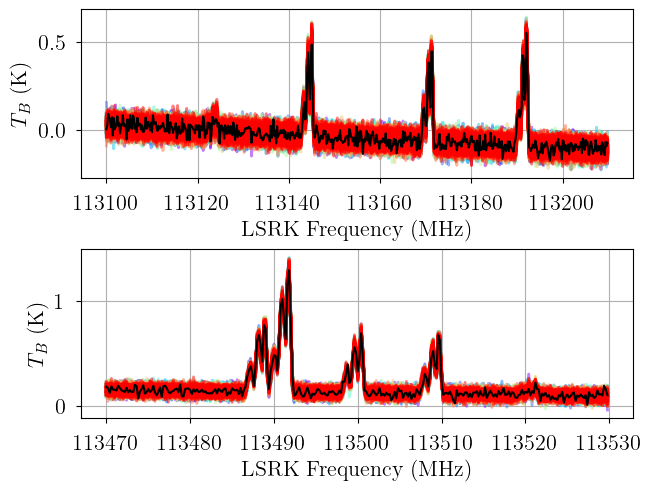
We generate posterior predictive checks as well as a trace plot of the individual chains. In the posterior predictive plot, we show each chain as a different color. Each line is one posterior sample.
[17]:
posterior = model.sample_posterior_predictive(
    thin=10, # keep one in {thin} posterior samples
)
_ = plot_predictive(model.data, posterior.posterior_predictive)
Sampling: [12CN-1, 12CN-2]
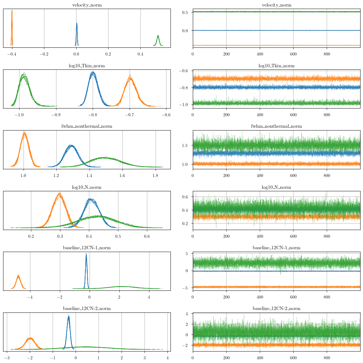
[18]:
from bayes_spec.plots import plot_traces

axes = plot_traces(model.trace.solution_0, model.cloud_freeRVs + model.baseline_freeRVs + model.hyper_freeRVs)
fig = axes.ravel()[0].figure
fig.tight_layout()
We can inspect the posterior distribution pair plots. The red points represent the simulation parameters.
[19]:
from bayes_spec.plots import plot_pair

# ignore transition and state dependent parameters
var_names = [
    param for param in model.cloud_deterministics
    if not set(model.model.named_vars_to_dims[param]).intersection(set(["transition", "state"]))
]
_ = plot_pair(
    model.trace.solution_0, # samples
    var_names, # var_names to plot
    labeller=model.labeller, # label manager
    kind="kde", # plot type
    reference_values=sim_params, # truths
)
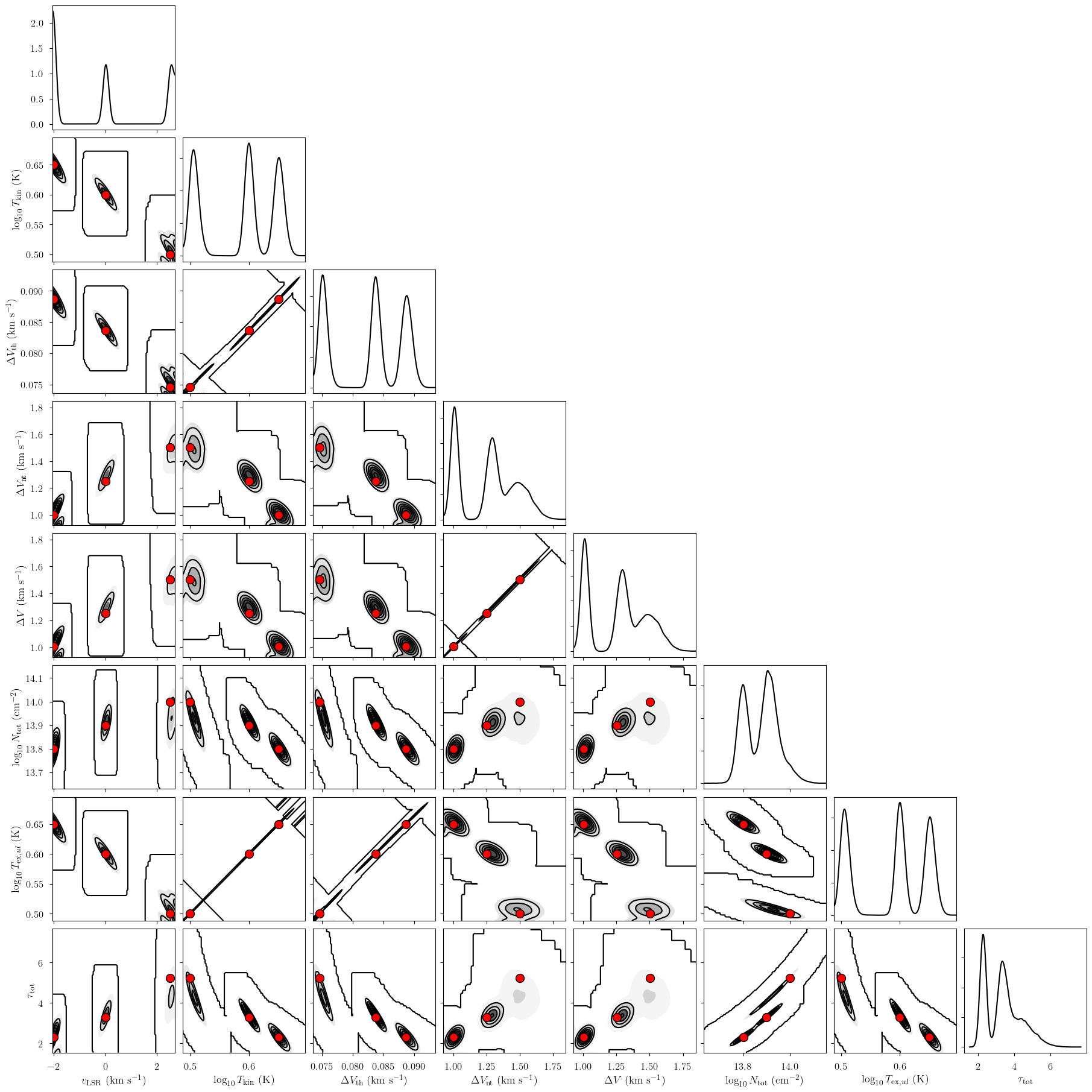
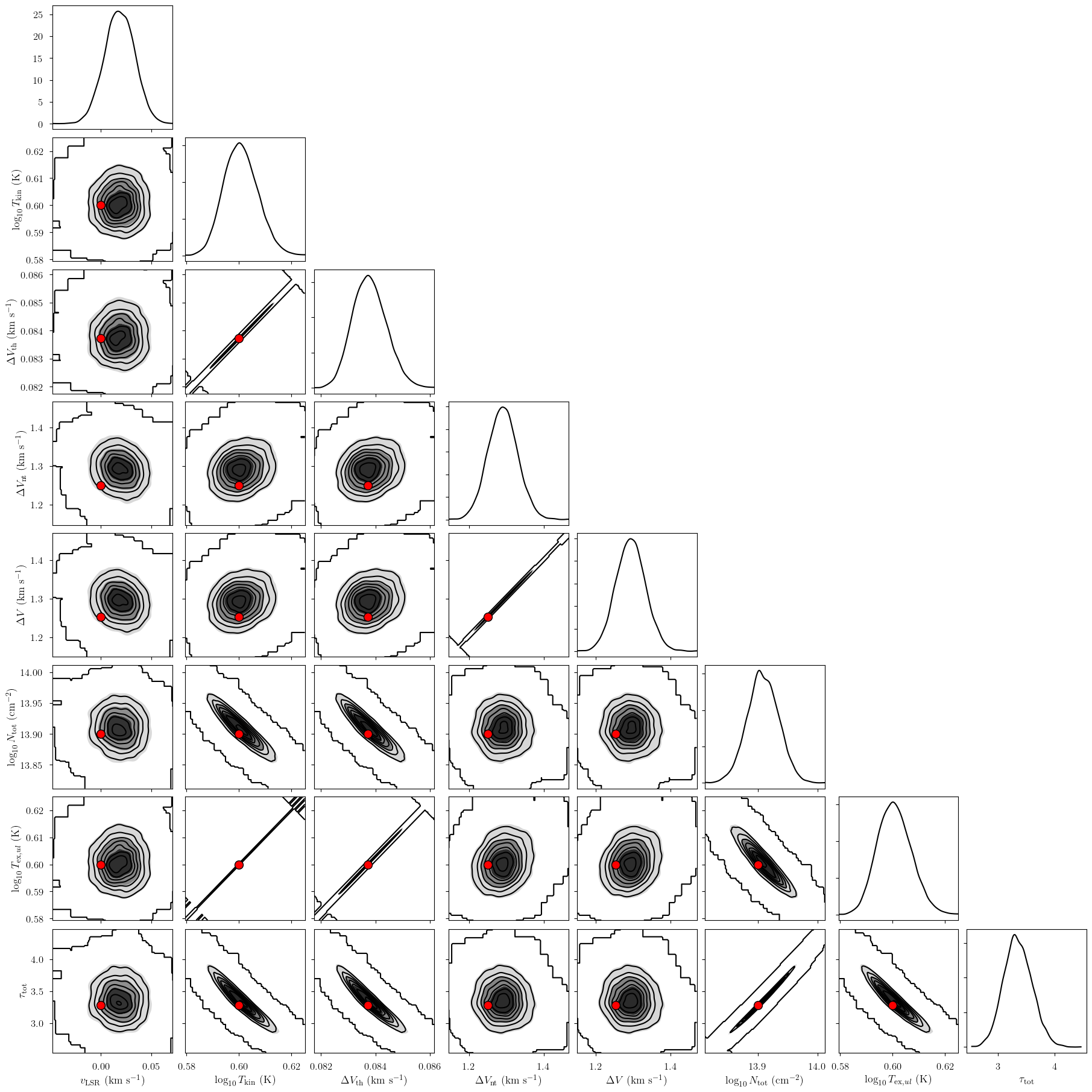
Notice that there are three posterior modes. These correspond to the three clouds of the model. We can plot the posterior distributions of the deterministic quantities for a single cloud (excluding the transition and state dependent parameters for clarity) along with the model hyper-parameters.
[20]:
# identify simulation cloud corresponding to each posterior cloud
sim_cloud_map = {}
for i in range(n_clouds):
    posterior_velocity = model.trace.solution_0['velocity'].sel(cloud=i).data.mean()
    match = np.argmin(np.abs(sim_params["velocity"] - posterior_velocity))
    sim_cloud_map[i] = match
sim_cloud_map
[20]:
{0: np.int64(1), 1: np.int64(0), 2: np.int64(2)}
[21]:
cloud = 0

# subset of sim_params
my_sim_params = {}
for var_name in model.cloud_deterministics:
    my_sim_params[var_name] = sim_params[var_name][sim_cloud_map[cloud]]

# ignore transition and state dependent parameters
var_names = [
    param for param in model.cloud_deterministics
    if not set(model.model.named_vars_to_dims[param]).intersection(set(["transition", "state"]))
]
_ = plot_pair(
    model.trace.solution_0.sel(cloud=cloud), # samples
    var_names, # var_names to plot
    labeller=model.labeller, # label manager
    kind="kde", # plot type
    reference_values=my_sim_params, # truths
)
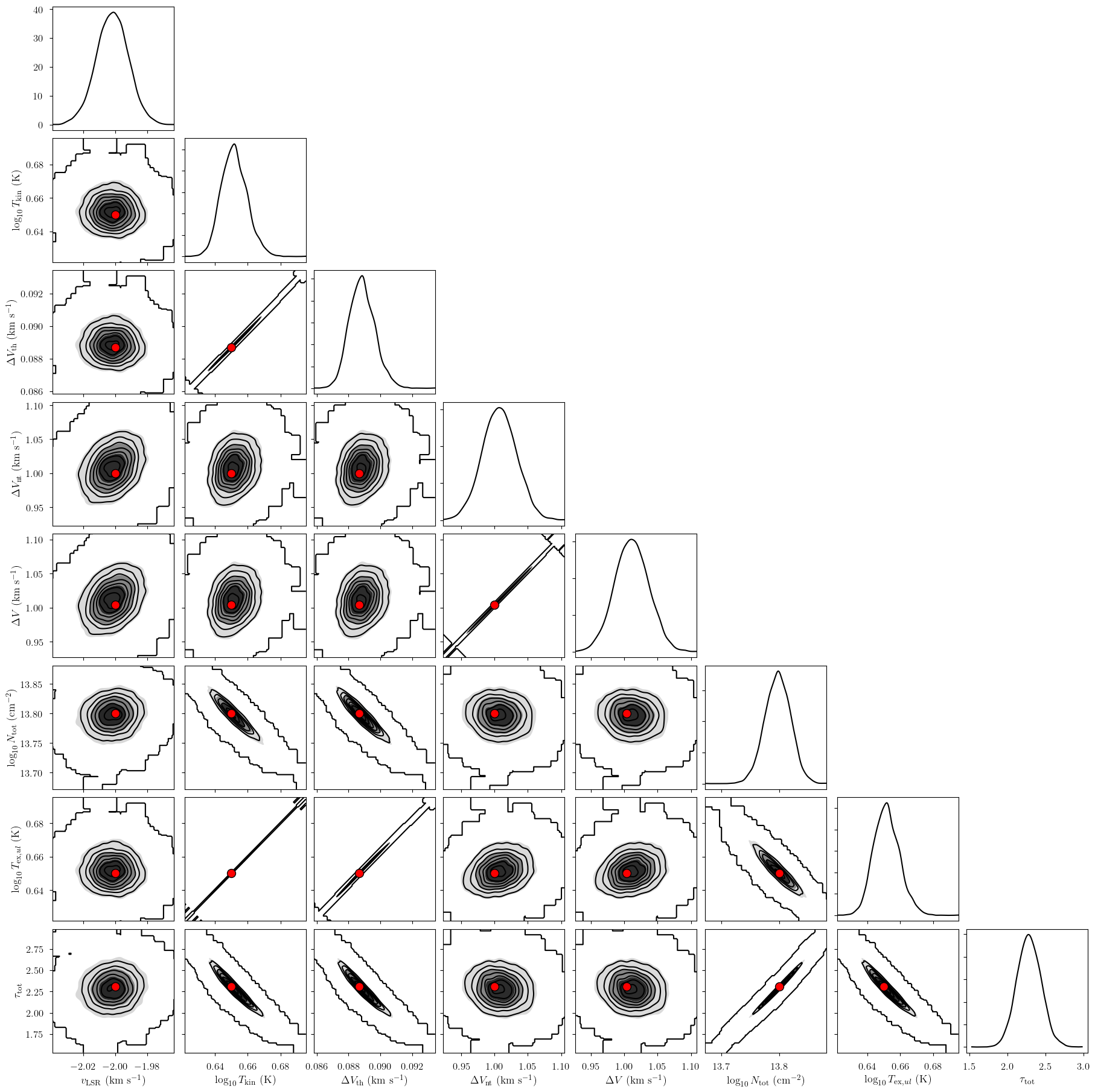
[22]:
cloud = 1

# subset of sim_params
my_sim_params = {}
for var_name in model.cloud_deterministics:
    my_sim_params[var_name] = sim_params[var_name][sim_cloud_map[cloud]]

# ignore transition and state dependent parameters
var_names = [
    param for param in model.cloud_deterministics
    if not set(model.model.named_vars_to_dims[param]).intersection(set(["transition", "state"]))
]
_ = plot_pair(
    model.trace.solution_0.sel(cloud=cloud), # samples
    var_names, # var_names to plot
    labeller=model.labeller, # label manager
    kind="kde", # plot type
    reference_values=my_sim_params, # truths
)
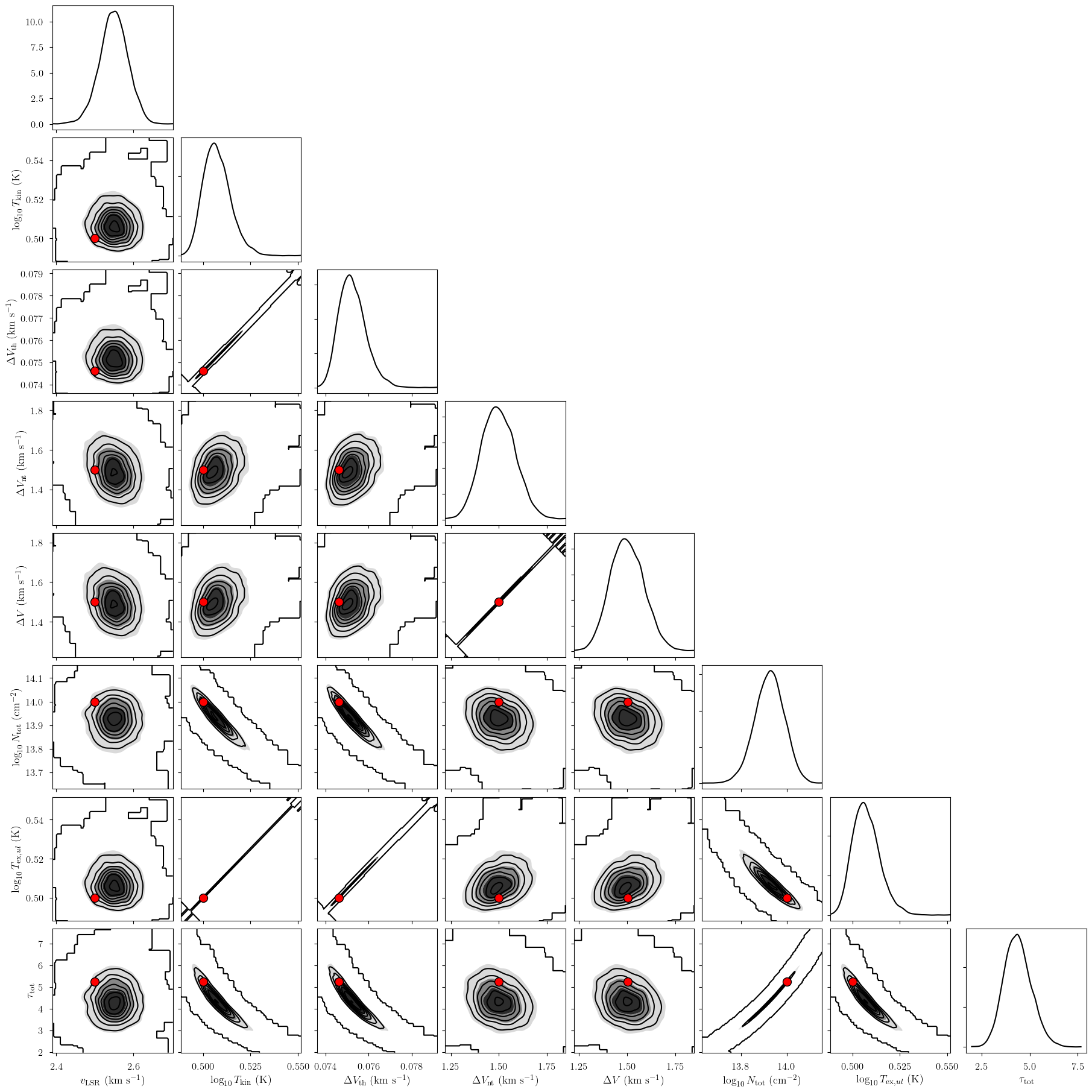
[23]:
cloud = 2

# subset of sim_params
my_sim_params = {}
for var_name in model.cloud_deterministics:
    my_sim_params[var_name] = sim_params[var_name][sim_cloud_map[cloud]]

# ignore transition and state dependent parameters
var_names = [
    param for param in model.cloud_deterministics
    if not set(model.model.named_vars_to_dims[param]).intersection(set(["transition", "state"]))
]
_ = plot_pair(
    model.trace.solution_0.sel(cloud=cloud), # samples
    var_names, # var_names to plot
    labeller=model.labeller, # label manager
    kind="kde", # plot type
    reference_values=my_sim_params, # truths
)
Finally, we can get the posterior statistics, Bayesian Information Criterion (BIC), etc.
[24]:
var_names=model.cloud_deterministics + model.baseline_freeRVs + model.hyper_deterministics
point_stats = az.summary(model.trace.solution_0, var_names=var_names, kind='stats', hdi_prob=0.68)
print("BIC:", model.bic())
display(point_stats)
BIC: -3441.9452824798577
| mean | sd | hdi_16% | hdi_84% | |
|---|---|---|---|---|
| velocity[0] | 0.019 | 0.015 | 0.005 | 0.035 |
| velocity[1] | -2.002 | 0.010 | -2.013 | -1.993 |
| velocity[2] | 2.549 | 0.036 | 2.513 | 2.584 |
| log10_Tkin[0] | 0.601 | 0.006 | 0.594 | 0.606 |
| log10_Tkin[1] | 0.652 | 0.008 | 0.644 | 0.659 |
| log10_Tkin[2] | 0.507 | 0.007 | 0.500 | 0.513 |
| fwhm_thermal[0] | 0.084 | 0.001 | 0.083 | 0.084 |
| fwhm_thermal[1] | 0.089 | 0.001 | 0.088 | 0.090 |
| fwhm_thermal[2] | 0.075 | 0.001 | 0.075 | 0.076 |
| fwhm_nonthermal[0] | 1.291 | 0.040 | 1.252 | 1.330 |
| fwhm_nonthermal[1] | 1.007 | 0.026 | 0.981 | 1.032 |
| fwhm_nonthermal[2] | 1.499 | 0.089 | 1.406 | 1.579 |
| fwhm[0] | 1.294 | 0.040 | 1.254 | 1.332 |
| fwhm[1] | 1.011 | 0.026 | 0.986 | 1.037 |
| fwhm[2] | 1.501 | 0.089 | 1.408 | 1.580 |
| log10_N[0] | 13.909 | 0.026 | 13.881 | 13.933 |
| log10_N[1] | 13.797 | 0.022 | 13.774 | 13.818 |
| log10_N[2] | 13.925 | 0.064 | 13.868 | 13.995 |
| log10_Tex_ul[0] | 0.601 | 0.006 | 0.594 | 0.606 |
| log10_Tex_ul[1] | 0.652 | 0.008 | 0.644 | 0.659 |
| log10_Tex_ul[2] | 0.507 | 0.007 | 0.500 | 0.513 |
| LTE_weights[0, 0 0 1 1] | 0.189 | 0.002 | 0.187 | 0.191 |
| LTE_weights[0, 0 0 1 2] | 0.377 | 0.003 | 0.375 | 0.381 |
| LTE_weights[0, 1 0 1 1] | 0.048 | 0.001 | 0.048 | 0.049 |
| LTE_weights[0, 1 0 1 2] | 0.097 | 0.001 | 0.095 | 0.098 |
| LTE_weights[0, 1 0 2 1] | 0.048 | 0.001 | 0.048 | 0.049 |
| LTE_weights[0, 1 0 2 2] | 0.096 | 0.001 | 0.095 | 0.097 |
| LTE_weights[0, 1 0 2 3] | 0.144 | 0.002 | 0.143 | 0.146 |
| LTE_weights[1, 0 0 1 1] | 0.176 | 0.002 | 0.175 | 0.178 |
| LTE_weights[1, 0 0 1 2] | 0.353 | 0.004 | 0.349 | 0.356 |
| LTE_weights[1, 1 0 1 1] | 0.053 | 0.001 | 0.052 | 0.053 |
| LTE_weights[1, 1 0 1 2] | 0.105 | 0.001 | 0.104 | 0.106 |
| LTE_weights[1, 1 0 2 1] | 0.052 | 0.001 | 0.052 | 0.053 |
| LTE_weights[1, 1 0 2 2] | 0.105 | 0.001 | 0.103 | 0.106 |
| LTE_weights[1, 1 0 2 3] | 0.157 | 0.002 | 0.155 | 0.159 |
| LTE_weights[2, 0 0 1 1] | 0.215 | 0.002 | 0.213 | 0.217 |
| LTE_weights[2, 0 0 1 2] | 0.429 | 0.004 | 0.426 | 0.434 |
| LTE_weights[2, 1 0 1 1] | 0.040 | 0.001 | 0.039 | 0.040 |
| LTE_weights[2, 1 0 1 2] | 0.079 | 0.001 | 0.078 | 0.081 |
| LTE_weights[2, 1 0 2 1] | 0.039 | 0.001 | 0.039 | 0.040 |
| LTE_weights[2, 1 0 2 2] | 0.079 | 0.001 | 0.077 | 0.080 |
| LTE_weights[2, 1 0 2 3] | 0.118 | 0.002 | 0.116 | 0.120 |
| Tex[113123.3687, 0] | 3.988 | 0.059 | 3.921 | 4.038 |
| Tex[113123.3687, 1] | 4.485 | 0.081 | 4.401 | 4.561 |
| Tex[113123.3687, 2] | 3.217 | 0.054 | 3.159 | 3.261 |
| Tex[113144.19, 0] | 3.988 | 0.059 | 3.921 | 4.038 |
| Tex[113144.19, 1] | 4.485 | 0.081 | 4.401 | 4.561 |
| Tex[113144.19, 2] | 3.217 | 0.054 | 3.159 | 3.261 |
| Tex[113170.535, 0] | 3.988 | 0.059 | 3.921 | 4.038 |
| Tex[113170.535, 1] | 4.485 | 0.081 | 4.401 | 4.561 |
| Tex[113170.535, 2] | 3.217 | 0.054 | 3.159 | 3.261 |
| Tex[113191.325, 0] | 3.988 | 0.059 | 3.921 | 4.038 |
| Tex[113191.325, 1] | 4.485 | 0.081 | 4.401 | 4.561 |
| Tex[113191.325, 2] | 3.217 | 0.054 | 3.159 | 3.261 |
| Tex[113488.142, 0] | 3.988 | 0.059 | 3.921 | 4.038 |
| Tex[113488.142, 1] | 4.485 | 0.081 | 4.401 | 4.561 |
| Tex[113488.142, 2] | 3.217 | 0.054 | 3.159 | 3.261 |
| Tex[113490.985, 0] | 3.988 | 0.059 | 3.921 | 4.038 |
| Tex[113490.985, 1] | 4.485 | 0.081 | 4.401 | 4.561 |
| Tex[113490.985, 2] | 3.217 | 0.054 | 3.159 | 3.261 |
| Tex[113499.643, 0] | 3.988 | 0.059 | 3.921 | 4.038 |
| Tex[113499.643, 1] | 4.485 | 0.081 | 4.401 | 4.561 |
| Tex[113499.643, 2] | 3.217 | 0.054 | 3.159 | 3.261 |
| Tex[113508.934, 0] | 3.988 | 0.059 | 3.921 | 4.038 |
| Tex[113508.934, 1] | 4.485 | 0.081 | 4.401 | 4.561 |
| Tex[113508.934, 2] | 3.217 | 0.054 | 3.159 | 3.261 |
| Tex[113520.4215, 0] | 3.988 | 0.059 | 3.921 | 4.038 |
| Tex[113520.4215, 1] | 4.485 | 0.081 | 4.401 | 4.561 |
| Tex[113520.4215, 2] | 3.217 | 0.054 | 3.159 | 3.261 |
| tau[113123.3687, 0] | 0.040 | 0.003 | 0.037 | 0.043 |
| tau[113123.3687, 1] | 0.028 | 0.002 | 0.026 | 0.029 |
| tau[113123.3687, 2] | 0.053 | 0.009 | 0.043 | 0.060 |
| tau[113144.19, 0] | 0.331 | 0.025 | 0.304 | 0.353 |
| tau[113144.19, 1] | 0.226 | 0.016 | 0.210 | 0.241 |
| tau[113144.19, 2] | 0.433 | 0.070 | 0.354 | 0.491 |
| tau[113170.535, 0] | 0.323 | 0.024 | 0.297 | 0.345 |
| tau[113170.535, 1] | 0.220 | 0.015 | 0.205 | 0.235 |
| tau[113170.535, 2] | 0.423 | 0.069 | 0.346 | 0.480 |
| tau[113191.325, 0] | 0.420 | 0.031 | 0.386 | 0.448 |
| tau[113191.325, 1] | 0.286 | 0.020 | 0.266 | 0.306 |
| tau[113191.325, 2] | 0.549 | 0.089 | 0.449 | 0.623 |
| tau[113488.142, 0] | 0.422 | 0.031 | 0.387 | 0.449 |
| tau[113488.142, 1] | 0.287 | 0.020 | 0.267 | 0.307 |
| tau[113488.142, 2] | 0.551 | 0.089 | 0.451 | 0.626 |
| tau[113490.985, 0] | 1.120 | 0.083 | 1.029 | 1.194 |
| tau[113490.985, 1] | 0.763 | 0.053 | 0.711 | 0.815 |
| tau[113490.985, 2] | 1.464 | 0.238 | 1.198 | 1.663 |
| tau[113499.643, 0] | 0.333 | 0.025 | 0.306 | 0.355 |
| tau[113499.643, 1] | 0.227 | 0.016 | 0.211 | 0.242 |
| tau[113499.643, 2] | 0.435 | 0.071 | 0.356 | 0.494 |
| tau[113508.934, 0] | 0.325 | 0.024 | 0.299 | 0.346 |
| tau[113508.934, 1] | 0.221 | 0.015 | 0.206 | 0.237 |
| tau[113508.934, 2] | 0.425 | 0.069 | 0.348 | 0.482 |
| tau[113520.4215, 0] | 0.041 | 0.003 | 0.037 | 0.043 |
| tau[113520.4215, 1] | 0.028 | 0.002 | 0.026 | 0.030 |
| tau[113520.4215, 2] | 0.053 | 0.009 | 0.043 | 0.060 |
| tau_total[0] | 3.355 | 0.248 | 3.082 | 3.576 |
| tau_total[1] | 2.285 | 0.159 | 2.128 | 2.443 |
| tau_total[2] | 4.387 | 0.712 | 3.585 | 4.977 |
| TR[113123.3687, 0] | 1.871 | 0.051 | 1.814 | 1.914 |
| TR[113123.3687, 1] | 2.306 | 0.072 | 2.231 | 2.373 |
| TR[113123.3687, 2] | 1.233 | 0.043 | 1.183 | 1.264 |
| TR[113144.19, 0] | 1.871 | 0.051 | 1.814 | 1.914 |
| TR[113144.19, 1] | 2.305 | 0.072 | 2.231 | 2.372 |
| TR[113144.19, 2] | 1.232 | 0.043 | 1.183 | 1.264 |
| TR[113170.535, 0] | 1.871 | 0.051 | 1.813 | 1.913 |
| TR[113170.535, 1] | 2.305 | 0.072 | 2.231 | 2.372 |
| TR[113170.535, 2] | 1.232 | 0.043 | 1.183 | 1.264 |
| TR[113191.325, 0] | 1.870 | 0.051 | 1.813 | 1.913 |
| TR[113191.325, 1] | 2.305 | 0.072 | 2.230 | 2.372 |
| TR[113191.325, 2] | 1.232 | 0.043 | 1.183 | 1.263 |
| TR[113488.142, 0] | 1.866 | 0.051 | 1.809 | 1.909 |
| TR[113488.142, 1] | 2.300 | 0.072 | 2.226 | 2.367 |
| TR[113488.142, 2] | 1.228 | 0.043 | 1.179 | 1.260 |
| TR[113490.985, 0] | 1.866 | 0.051 | 1.809 | 1.909 |
| TR[113490.985, 1] | 2.300 | 0.072 | 2.226 | 2.367 |
| TR[113490.985, 2] | 1.228 | 0.043 | 1.179 | 1.260 |
| TR[113499.643, 0] | 1.866 | 0.051 | 1.809 | 1.909 |
| TR[113499.643, 1] | 2.300 | 0.072 | 2.226 | 2.367 |
| TR[113499.643, 2] | 1.228 | 0.043 | 1.179 | 1.260 |
| TR[113508.934, 0] | 1.866 | 0.051 | 1.809 | 1.908 |
| TR[113508.934, 1] | 2.300 | 0.072 | 2.226 | 2.367 |
| TR[113508.934, 2] | 1.228 | 0.043 | 1.179 | 1.260 |
| TR[113520.4215, 0] | 1.866 | 0.051 | 1.809 | 1.908 |
| TR[113520.4215, 1] | 2.300 | 0.072 | 2.225 | 2.367 |
| TR[113520.4215, 2] | 1.228 | 0.043 | 1.179 | 1.260 |
| baseline_12CN-1_norm[0] | -0.214 | 0.053 | -0.266 | -0.160 |
| baseline_12CN-1_norm[1] | -4.779 | 0.141 | -4.913 | -4.628 |
| baseline_12CN-1_norm[2] | 2.186 | 0.793 | 1.398 | 2.983 |
| baseline_12CN-2_norm[0] | -0.316 | 0.071 | -0.387 | -0.248 |
| baseline_12CN-2_norm[1] | -1.990 | 0.202 | -2.187 | -1.788 |
| baseline_12CN-2_norm[2] | 0.433 | 0.888 | -0.358 | 1.435 |
[ ]: