WB89_380

Trey V. Wenger - March 2025

# General imports
import os
import pickle
import time

import matplotlib.pyplot as plt
import arviz as az
import pandas as pd
import numpy as np
import pymc as pm

print("arviz version:", az.__version__)

print("pymc version:", pm.__version__)

import bayes_spec
print("bayes_spec version:", bayes_spec.__version__)

import bayes_cn_hfs
print("bayes_cn_hfs version:", bayes_cn_hfs.__version__)

# Notebook configuration
pd.options.display.max_rows = None

arviz version: 0.22.0dev
pymc version: 5.21.1
bayes_spec version: 1.7.5
bayes_cn_hfs version: 1.1.1+9.gf278c50.dirty

Load the data

from bayes_spec import SpecData

data_12CN = np.genfromtxt("12CN_WB89_380_freq.dat")
data_13CN = np.genfromtxt("13CN_WB89_380_freq.dat")

# estimate noise
noise_12CN = 1.4826 * np.median(np.abs(data_12CN[:, 1] - np.median(data_12CN[:, 1])))
print("rms 12CN", noise_12CN)
noise_13CN = 1.4826 * np.median(np.abs(data_13CN[:, 1] - np.median(data_13CN[:, 1])))
print("rms 13CN", noise_13CN)

# boxcar smooth 13CN to 4 channels
data_13CN_smo_x = data_13CN[:, 0].reshape(93, 4).mean(axis=1)
data_13CN_smo = data_13CN[:, 1].reshape(93, 4).mean(axis=1)

obs_12CN_1 = SpecData(
    data_12CN[0:600, 0],
    data_12CN[0:600, 1],
    noise_12CN,
    xlabel=r"LSRK Frequency (MHz)",
    ylabel=r"$T_A^*$ (K)",
)
obs_12CN_2 = SpecData(
    data_12CN[-500:-1, 0],
    data_12CN[-500:-1, 1],
    noise_12CN,
    xlabel=r"LSRK Frequency (MHz)",
    ylabel=r"$T_A^*$ (K)",
)
obs_13CN_1 = SpecData(
    data_13CN[:, 0],
    data_13CN[:, 1],
    noise_13CN,
    xlabel=r"LSRK Frequency (MHz)",
    ylabel=r"$T_A^*$ (K)",
)
obs_13CN_2 = SpecData(
    data_13CN_smo_x,
    data_13CN_smo,
    noise_13CN,
    xlabel=r"LSRK Frequency (MHz)",
    ylabel=r"Smoothed $T_A^*$ (K)",
)
data = {"12CN-1": obs_12CN_1, "12CN-2": obs_12CN_2, "13CN-1": obs_13CN_1, "13CN-2": obs_13CN_2}

# subset of 12CN data
data_12CN = {
    label: data[label]
    for label in data.keys() if "12CN" in label
}

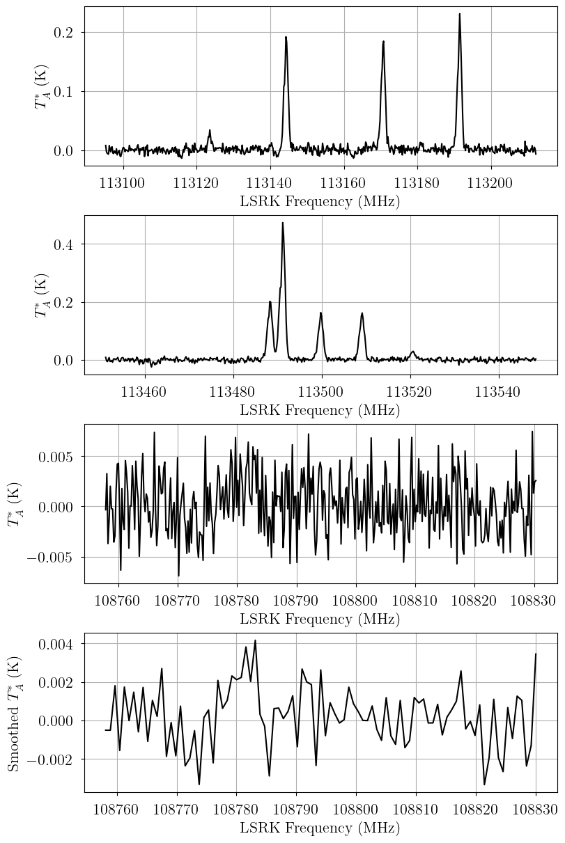
# Plot the data
fig, axes = plt.subplots(len(data), layout="constrained", figsize=(8, 12))
for i, label in enumerate(data.keys()):
    axes[i].plot(data[label].spectral, data[label].brightness, 'k-')
    axes[i].set_xlabel(data[label].xlabel)
    axes[i].set_ylabel(data[label].ylabel)

rms 12CN 0.005452432119031414
rms 13CN 0.0029468342287699194

Reproduce Sun et al. (2024) model

import astropy.units as u
import astropy.constants as c
from bayes_cn_hfs.utils import supplement_mol_data
from bayes_cn_hfs.physics import calc_stat_weight

mol_data_12CN, weight_12CN = supplement_mol_data("CN")

sun2024_tau_ml = 0.58
sun2024_Tex = 4.34*u.K
freq = 113.5*u.GHz

# main line upper state column density
sun2024_Nu_ml = 8.0*np.pi*freq**2.0 / c.c**2.0 / (np.exp(c.h*freq/(c.k_B*sun2024_Tex)) - 1.0) / (mol_data_12CN["Aul"][5]/u.s) / (1.0/u.MHz) * sun2024_tau_ml
print("main line log10 upper column density", np.log10(sun2024_Nu_ml.to('cm-2').value))

# partition function
stat_weights = calc_stat_weight(mol_data_12CN["states"]["deg"], mol_data_12CN["states"]["E"], sun2024_Tex.to("K").value).eval()
Qtot = np.sum(stat_weights)

# total column density
sun2024_log10_Ntot = np.log10(Qtot/stat_weights[6] * sun2024_Nu_ml.to('cm-2').value)
print("log10 total column density", sun2024_log10_Ntot)

main line log10 upper column density 12.849858056215492
log10 total column density 13.663493893907637

from bayes_cn_hfs.cn_model import CNModel

# Initialize and define the model
baseline_degree = 0
n_clouds = 1
model = CNModel(
    data_12CN,
    molecule="CN", # molecule (either "CN" or "13CN")
    mol_data=mol_data_12CN, # molecular data
    bg_temp = 2.7, # assumed background temperature (K)
    Beff=0.78, # Main beam efficiency
    Feff=0.94, # Forward efficiency
    n_clouds=n_clouds,
    baseline_degree=baseline_degree,
    seed=1234,
    verbose=True
)
model.add_priors(
    prior_log10_N = [13.5, 1.0], # mean and width of log10 total column density prior (cm-2)
    prior_log10_Tkin = [1.0, 0.5], # mean and width of log10 kinetic temperature prior (K)
    prior_velocity = [0.0, 3.0], # mean and width of velocity prior (km/s)
    prior_fwhm_nonthermal = 1.0, # width of non-thermal broadening prior (km/s)
    prior_fwhm_L = None, # assume Gaussian line profile
    prior_rms = None, # do not infer spectral rms
    prior_baseline_coeffs = None, # use default baseline priors
    assume_LTE = True, # assume LTE
    prior_log10_Tex = [0.5, 0.1], # ignored because LTE
    assume_CTEX = True, # implied because LTE
    prior_LTE_precision = 100.0, # ignored because LTE
    fix_log10_Tkin = None, # do not fix the kinetic temperature
    ordered = False, # do not assume optically-thin
)
model.add_likelihood()

# Simulate with Sun et al. (2024) parameters
# We choose values for velocity and FWHM that look good
sim_params = {
    "log10_N": [sun2024_log10_Ntot],
    "log10_Tkin": [np.log10(sun2024_Tex.to("K").value)],
    "fwhm_nonthermal": [2.75],
    "velocity": [-0.5],
    "fwhm_L": 0.0,
    "rms_12CN-1": 0.0,
    "rms_12CN-2": 0.0,
    "baseline_12CN-1_norm": [0.0],
    "baseline_12CN-2_norm": [0.0],
}

# add derived quantities to sim_params
for key in model.cloud_deterministics:
    if key not in sim_params.keys():
        sim_params[key] = model.model[key].eval(sim_params, on_unused_input="ignore")

# Evaluate and save simulated observations
sim_obs = {label: model.model[label].eval(sim_params, on_unused_input="ignore") for label in data_12CN.keys()}

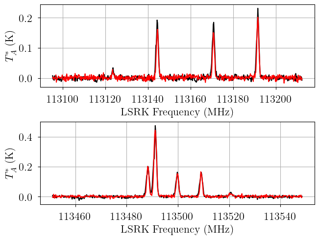
# Plot the simulated data
fig, axes = plt.subplots(len(data_12CN), layout="constrained")
for i, label in enumerate(data_12CN.keys()):
    axes[i].plot(data_12CN[label].spectral, data_12CN[label].brightness, 'k-')
    axes[i].plot(data_12CN[label].spectral, sim_obs[label], 'r-')
    axes[i].set_xlabel(data_12CN[label].xlabel)
    axes[i].set_ylabel(data_12CN[label].ylabel)

sim_params

{'log10_N': [np.float64(13.663493893907637)],
 'log10_Tkin': [np.float64(0.6374897295125107)],
 'fwhm_nonthermal': [2.75],
 'velocity': [-0.5],
 'fwhm_L': 0.0,
 'rms_12CN-1': 0.0,
 'rms_12CN-2': 0.0,
 'baseline_12CN-1_norm': [0.0],
 'baseline_12CN-2_norm': [0.0],
 'fwhm_thermal': array([0.08740951]),
 'fwhm': array([2.75138882]),
 'log10_Tex_ul': array([0.63748973]),
 'Tex': array([[4.34],
        [4.34],
        [4.34],
        [4.34],
        [4.34],
        [4.34],
        [4.34],
        [4.34],
        [4.34]]),
 'tau': array([[0.02095209],
        [0.17150941],
        [0.16750926],
        [0.21752014],
        [0.21834459],
        [0.58001127],
        [0.17227444],
        [0.16830736],
        [0.02105628]]),
 'tau_total': array([1.73748484]),
 'TR': array([[2.17718756],
        [2.17688599],
        [2.17650447],
        [2.17620343],
        [2.17190905],
        [2.17186795],
        [2.17174278],
        [2.17160848],
        [2.17144243]])}

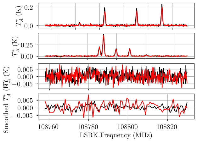
This simulation is consistent with the Sun et al. (2024) model, but it is not a great fit to the data.

from bayes_cn_hfs import CNRatioModel

sun2024_ratio_12C_13C = 57.0

baseline_degree = 0
n_clouds = 1
model = CNRatioModel(
    data,
    bg_temp = 2.7, # assumed background temperature (K)
    Beff=0.78, # Main beam efficiency
    Feff=0.94, # Forward efficiency
    n_clouds=n_clouds,
    baseline_degree=baseline_degree,
    seed=1234,
    verbose=True
)
model.add_priors(
    prior_log10_N_12CN = [13.5, 1.0], # mean and width of log10 12CN total column density prior (cm-2)
    prior_ratio_12C_13C = [75.0, 25.0], # mean and width of 12C/13C ratio prior
    prior_log10_Tkin = [1.0, 0.5], # mean and width of log10 kinetic temperature prior (K)
    prior_velocity = [0.0, 3.0], # mean and width of velocity prior (km/s)
    prior_fwhm_nonthermal = 1.0, # width of non-thermal broadening prior (km/s)
    prior_fwhm_L = None, # assume Gaussian line profile
    prior_rms = None, # do not infer spectral rms
    prior_baseline_coeffs = None, # use default baseline priors
    assume_LTE = True, # assume LTE
    prior_log10_Tex = None, # ignored for this LTE model
    assume_CTEX_12CN = True, # implied for this LTE model
    prior_LTE_precision = 100.0, # ignored for this LTE model
    assume_CTEX_13CN = True, # implied for this LTE model
    fix_log10_Tkin = None, # do not fix the kinetic temperature
    ordered = False, # do not assume optically-thin
)
model.add_likelihood()

# Simulate with Sun et al. (2024) parameters
# We choose values for velocity and FWHM that look good
sim_params = {
    "log10_N_12CN": [sun2024_log10_Ntot],
    "log10_Tkin": [np.log10(sun2024_Tex.to("K").value)],
    "fwhm_nonthermal": [2.75],
    "velocity": [-0.5],
    "fwhm_L": 0.0,
    "rms_12CN-1": 0.0,
    "rms_12CN-2": 0.0,
    "rms_13CN-1": 0.0,
    "rms_13CN-2": 0.0,
    "baseline_12CN-1_norm": [0.0],
    "baseline_12CN-2_norm": [0.0],
    "baseline_13CN-1_norm": [0.0],
    "baseline_13CN-2_norm": [0.0],
}

# add derived quantities to sim_params
for key in model.cloud_deterministics:
    if key not in sim_params.keys():
        sim_params[key] = model.model[key].eval(sim_params, on_unused_input="ignore")

# Evaluate and save simulated observations
sim_obs = {key: model.model[key].eval(sim_params, on_unused_input="ignore") for key in data.keys()}

# Plot the simulated data
fig, axes = plt.subplots(len(data.keys()))
for ax, key in zip(axes, data.keys()):
    ax.plot(data[key].spectral, data[key].brightness, "k-")
    ax.plot(data[key].spectral, sim_obs[key], "r-")
    ax.set_xlabel(data[key].xlabel)
    ax.set_ylabel(data[key].ylabel)

sim_params

{'log10_N_12CN': [np.float64(13.663493893907637)],
 'log10_Tkin': [np.float64(0.6374897295125107)],
 'fwhm_nonthermal': [2.75],
 'velocity': [-0.5],
 'fwhm_L': 0.0,
 'rms_12CN-1': 0.0,
 'rms_12CN-2': 0.0,
 'rms_13CN-1': 0.0,
 'rms_13CN-2': 0.0,
 'baseline_12CN-1_norm': [0.0],
 'baseline_12CN-2_norm': [0.0],
 'baseline_13CN-1_norm': [0.0],
 'baseline_13CN-2_norm': [0.0],
 'fwhm_thermal_12CN': array([0.08740951]),
 'fwhm_thermal_13CN': array([0.08577554]),
 'fwhm_12CN': array([2.75138882]),
 'fwhm_13CN': array([2.75133739]),
 'N_13CN': array([3.95063481e+11]),
 'log10_Tex_ul': array([0.63748973]),
 'Tex_12CN': array([[4.34],
        [4.34],
        [4.34],
        [4.34],
        [4.34],
        [4.34],
        [4.34],
        [4.34],
        [4.34]]),
 'tau_12CN': array([[0.02095209],
        [0.17150941],
        [0.16750926],
        [0.21752014],
        [0.21834459],
        [0.58001127],
        [0.17227444],
        [0.16830736],
        [0.02105628]]),
 'tau_total_12CN': array([1.73748484]),
 'TR_12CN': array([[2.17718756],
        [2.17688599],
        [2.17650447],
        [2.17620343],
        [2.17190905],
        [2.17186795],
        [2.17174278],
        [2.17160848],
        [2.17144243]]),
 'Tex_13CN': array([[4.34],
        [4.34],
        [4.34],
        [4.34],
        [4.34],
        [4.34],
        [4.34],
        [4.34],
        [4.34],
        [4.34],
        [4.34],
        [4.34],
        [4.34],
        [4.34],
        [4.34],
        [4.34],
        [4.34],
        [4.34],
        [4.34],
        [4.34],
        [4.34],
        [4.34],
        [4.34],
        [4.34],
        [4.34],
        [4.34],
        [4.34],
        [4.34]]),
 'tau_13CN': array([[2.42835648e-05],
        [3.16703709e-05],
        [1.23408989e-05],
        [5.47863821e-05],
        [3.31676646e-05],
        [8.89079759e-05],
        [1.02529302e-04],
        [3.41650731e-04],
        [6.81880498e-04],
        [3.48554637e-04],
        [1.04945647e-03],
        [3.89948783e-04],
        [4.62104220e-04],
        [3.46448331e-04],
        [2.97537399e-04],
        [1.78005131e-03],
        [1.30666953e-03],
        [3.61300093e-04],
        [2.65422406e-03],
        [1.39886790e-03],
        [6.18907003e-04],
        [4.83459062e-04],
        [4.96709732e-04],
        [3.50498034e-05],
        [6.00206687e-06],
        [1.24841502e-04],
        [3.23711079e-05],
        [8.74301190e-05]]),
 'tau_total_13CN': array([0.01365115]),
 'TR_13CN': array([[2.25156137],
        [2.25154682],
        [2.25146073],
        [2.25125198],
        [2.2512473 ],
        [2.25103856],
        [2.24636192],
        [2.24626152],
        [2.24605331],
        [2.24302354],
        [2.24293752],
        [2.2429184 ],
        [2.24283867],
        [2.24282725],
        [2.24281681],
        [2.24272441],
        [2.24263028],
        [2.24261098],
        [2.24081397],
        [2.24078178],
        [2.24071351],
        [2.24061319],
        [2.24057398],
        [2.24040509],
        [2.2377537 ],
        [2.23434092],
        [2.23432968],
        [2.23432098]])}

Ratio Model

We fix the kinetic temperature at the Sun et al. (2024) model value and assume LTE.

from bayes_cn_hfs import CNRatioModel

# Initialize and define the model
baseline_degree = 0
n_clouds = 1
model = CNRatioModel(
    data,
    bg_temp = 2.7, # assumed background temperature (K)
    Beff=0.78, # Main beam efficiency
    Feff=0.94, # Forward efficiency
    n_clouds=n_clouds,
    baseline_degree=baseline_degree,
    seed=1234,
    verbose=True
)
model.add_priors(
    prior_log10_N_12CN = [13.5, 1.0], # mean and width of log10 12CN total column density prior (cm-2)
    prior_ratio_12C_13C = [75.0, 25.0], # mean and width of 12C/13C ratio prior
    prior_log10_Tkin = [1.0, 0.5], # mean and width of log10 kinetic temperature prior (K)
    prior_velocity = [0.0, 3.0], # mean and width of velocity prior (km/s)
    prior_fwhm_nonthermal = 1.0, # width of non-thermal broadening prior (km/s)
    prior_fwhm_L = None, # assume Gaussian line profile
    prior_rms = None, # do not infer spectral rms
    prior_baseline_coeffs = None, # use default baseline priors
    assume_LTE = True, # assume LTE
    prior_log10_Tex = None, # ignored for this LTE model
    assume_CTEX_12CN = True, # implied for this LTE model
    prior_LTE_precision = 100.0, # ignored for this LTE model
    assume_CTEX_13CN = True, # implied for this LTE model
    fix_log10_Tkin = np.log10(sun2024_Tex.to("K").value), # fix the kinetic (excitation) temperature
    ordered = False, # do not assume optically-thin
)
model.add_likelihood()

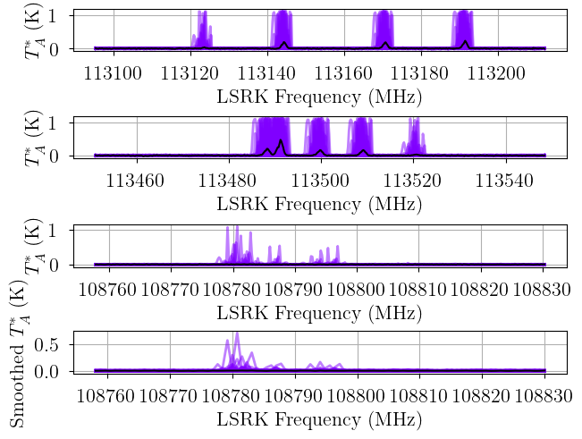
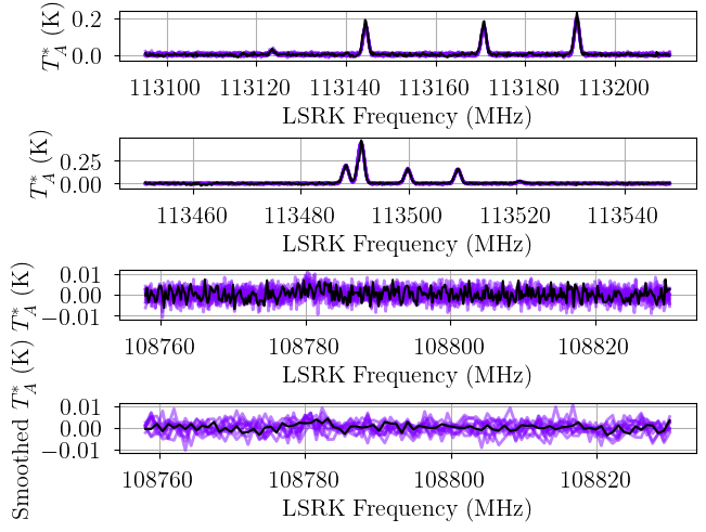
from bayes_spec.plots import plot_predictive

# prior predictive check
prior = model.sample_prior_predictive(
    samples=100,  # prior predictive samples
)
_ = plot_predictive(model.data, prior.prior_predictive)

Sampling: [12CN-1, 12CN-2, 13CN-1, 13CN-2, baseline_12CN-1_norm, baseline_12CN-2_norm, baseline_13CN-1_norm, baseline_13CN-2_norm, fwhm_nonthermal_norm, log10_N_12CN_norm, ratio_12C_13C, velocity_norm]

start = time.time()
model.fit(
    n = 100_000, # maximum number of VI iterations
    draws = 1_000, # number of posterior samples
    rel_tolerance = 0.01, # VI relative convergence threshold
    abs_tolerance = 0.1, # VI absolute convergence threshold
    learning_rate = 0.02, # VI learning rate
)
end = time.time()
print(f"Runtime: {(end-start)/60.0:.2f} minutes")

Convergence achieved at 2000
Interrupted at 1,999 [1%]: Average Loss = 731.11

Runtime: 0.41 minutes

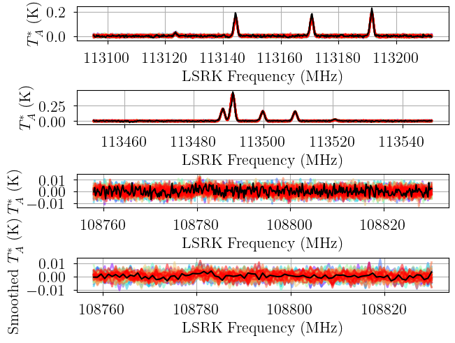
posterior = model.sample_posterior_predictive(
    thin=100, # keep one in {thin} posterior samples
)
_ = plot_predictive(model.data, posterior.posterior_predictive)

Sampling: [12CN-1, 12CN-2, 13CN-1, 13CN-2]

start = time.time()
init_kwargs = {
    "rel_tolerance": 0.01,
    "abs_tolerance": 0.1,
    "learning_rate": 0.02,
}
model.sample(
    init = "advi+adapt_diag", # initialization strategy
    tune = 1000, # tuning samples
    draws = 1000, # posterior samples
    chains = 8, # number of independent chains
    cores = 8, # number of parallel chains
    init_kwargs = init_kwargs, # VI initialization arguments
    nuts_kwargs = {"target_accept": 0.8}, # NUTS arguments
)
end = time.time()
print(f"Runtime: {(end-start)/60.0:.2f} minutes")

Initializing NUTS using custom advi+adapt_diag strategy

Convergence achieved at 2000
Interrupted at 1,999 [1%]: Average Loss = 731.11
Multiprocess sampling (8 chains in 8 jobs)
NUTS: [baseline_12CN-1_norm, baseline_12CN-2_norm, baseline_13CN-1_norm, baseline_13CN-2_norm, velocity_norm, fwhm_nonthermal_norm, log10_N_12CN_norm, ratio_12C_13C]

Sampling 8 chains for 1_000 tune and 1_000 draw iterations (8_000 + 8_000 draws total) took 17 seconds.

Adding log-likelihood to trace

Runtime: 0.82 minutes

model.solve(kl_div_threshold=0.1)

GMM converged to unique solution

posterior = model.sample_posterior_predictive(
    thin=100, # keep one in {thin} posterior samples
)
_ = plot_predictive(model.data, posterior.posterior_predictive)

Sampling: [12CN-1, 12CN-2, 13CN-1, 13CN-2]

print("solutions:", model.solutions)

# ignore transition and state dependent parameters
var_names = [
    param for param in model.cloud_deterministics
    if not set(model.model.named_vars_to_dims[param]).intersection(set(
        ["transition_12CN", "state_12CN", "transition_13CN", "state_13CN"]
    ))
]
pm.summary(model.trace.posterior, var_names=var_names + model.hyper_deterministics + model.baseline_freeRVs + ["ratio_12C_13C"])

solutions: [0]

/home/twenger/miniconda3/envs/bayes_spec-dev/lib/python3.13/site-packages/arviz/stats/diagnostics.py:596: RuntimeWarning: invalid value encountered in scalar divide
  (between_chain_variance / within_chain_variance + num_samples - 1) / (num_samples)
/home/twenger/miniconda3/envs/bayes_spec-dev/lib/python3.13/site-packages/arviz/stats/diagnostics.py:991: RuntimeWarning: invalid value encountered in scalar divide
  varsd = varvar / evar / 4
/home/twenger/miniconda3/envs/bayes_spec-dev/lib/python3.13/site-packages/arviz/stats/diagnostics.py:596: RuntimeWarning: invalid value encountered in scalar divide
  (between_chain_variance / within_chain_variance + num_samples - 1) / (num_samples)

	mean	sd	hdi_3%	hdi_97%	mcse_mean	mcse_sd	ess_bulk	ess_tail	r_hat
velocity[0]	-4.660000e-01	9.000000e-03	-4.820000e-01	-4.500000e-01	0.000000e+00	0.000000e+00	10037.0	6544.0	1.0
fwhm_thermal_12CN[0]	8.700000e-02	0.000000e+00	8.700000e-02	8.700000e-02	0.000000e+00	NaN	8000.0	8000.0	NaN
fwhm_thermal_13CN[0]	8.600000e-02	0.000000e+00	8.600000e-02	8.600000e-02	0.000000e+00	0.000000e+00	8000.0	8000.0	NaN
fwhm_nonthermal[0]	3.263000e+00	2.000000e-02	3.227000e+00	3.301000e+00	0.000000e+00	0.000000e+00	7629.0	6356.0	1.0
fwhm_12CN[0]	3.265000e+00	2.000000e-02	3.228000e+00	3.302000e+00	0.000000e+00	0.000000e+00	7629.0	6356.0	1.0
fwhm_13CN[0]	3.265000e+00	2.000000e-02	3.228000e+00	3.302000e+00	0.000000e+00	0.000000e+00	7629.0	6356.0	1.0
log10_N_12CN[0]	1.372800e+01	2.000000e-03	1.372400e+01	1.373200e+01	0.000000e+00	0.000000e+00	7216.0	6121.0	1.0
N_13CN[0]	6.963536e+11	1.368538e+11	4.521969e+11	9.556013e+11	1.443470e+09	1.491232e+09	8889.0	6392.0	1.0
log10_Tex_ul[0]	6.370000e-01	0.000000e+00	6.370000e-01	6.370000e-01	0.000000e+00	0.000000e+00	8000.0	8000.0	NaN
tau_total_12CN[0]	2.017000e+00	1.100000e-02	1.996000e+00	2.036000e+00	0.000000e+00	0.000000e+00	7216.0	6121.0	1.0
tau_total_13CN[0]	2.400000e-02	5.000000e-03	1.600000e-02	3.300000e-02	0.000000e+00	0.000000e+00	8889.0	6392.0	1.0
baseline_12CN-1_norm[0]	7.000000e-03	4.100000e-02	-6.900000e-02	8.400000e-02	0.000000e+00	0.000000e+00	8729.0	6114.0	1.0
baseline_12CN-2_norm[0]	-2.980000e-01	4.700000e-02	-3.860000e-01	-2.100000e-01	1.000000e-03	1.000000e-03	8960.0	5859.0	1.0
baseline_13CN-1_norm[0]	2.100000e-02	5.300000e-02	-8.200000e-02	1.170000e-01	1.000000e-03	1.000000e-03	10375.0	6784.0	1.0
baseline_13CN-2_norm[0]	-8.600000e-02	1.020000e-01	-2.860000e-01	9.600000e-02	1.000000e-03	1.000000e-03	10346.0	6116.0	1.0
ratio_12C_13C[0]	7.988900e+01	1.637600e+01	5.213900e+01	1.107800e+02	1.790000e-01	2.200000e-01	8883.0	6487.0	1.0

We find a slightly larger \(^{12}{\rm C}/^{13}{\rm C}\) ratio: \(80 \pm 16\) compared to Sun et al. (2024) who found \(57 \pm 17\) using the traditional HfS method and \(57 \pm 13\) using the satellite-line method.

Single component LTE

Mimic Sun et al. (2024) analysis.

# Initialize and define the model
baseline_degree = 0
n_clouds = 1
model = CNModel(
    data_12CN,
    molecule="CN", # molecule (either "CN" or "13CN")
    mol_data=mol_data_12CN, # molecular data
    bg_temp = 2.7, # assumed background temperature (K)
    Beff=0.78, # Main beam efficiency
    Feff=0.94, # Forward efficiency
    n_clouds=n_clouds,
    baseline_degree=baseline_degree,
    seed=1234,
    verbose=True
)
model.add_priors(
    prior_log10_N = [13.75, 0.25], # mean and width of log10 total column density prior (cm-2)
    prior_log10_Tkin = [0.75, 0.25], # mean and width of log10 kinetic temperature prior (K)
    prior_velocity = [0.0, 3.0], # mean and width of velocity prior (km/s)
    prior_fwhm_nonthermal = 1.0, # width of non-thermal broadening prior (km/s)
    prior_fwhm_L = 1.0, # width of latent Lorentzian FWHM prior (km/s) TIP: set to typical feature separation
    prior_rms = None, # do not infer spectral rms
    prior_baseline_coeffs = None, # use default baseline priors
    assume_LTE = True, # assume LTE
    prior_log10_Tex = [0.75, 0.25], # ignored because LTE
    assume_CTEX = True, # implied because LTE
    prior_LTE_precision = 100.0, # ignored because LTE
    fix_log10_Tkin = None, # do not fix the kinetic temperature
    ordered = False, # do not assume optically-thin
)
model.add_likelihood()

from bayes_spec.plots import plot_predictive

# prior predictive check
prior = model.sample_prior_predictive(
    samples=100,  # prior predictive samples
)
_ = plot_predictive(model.data, prior.prior_predictive)

start = time.time()
model.fit(
    n = 100_000, # maximum number of VI iterations
    draws = 1_000, # number of posterior samples
    rel_tolerance = 0.01, # VI relative convergence threshold
    abs_tolerance = 0.1, # VI absolute convergence threshold
    learning_rate = 0.02, # VI learning rate
)
end = time.time()
print(f"Runtime: {(end-start)/60.0:.2f} minutes")

posterior = model.sample_posterior_predictive(
    thin=100, # keep one in {thin} posterior samples
)
_ = plot_predictive(model.data, posterior.posterior_predictive)

pm.summary(model.trace.posterior)

start = time.time()
model.sample(
    init = "advi+adapt_diag", # initialization strategy
    tune = 1000, # tuning samples
    draws = 1000, # posterior samples
    chains = 8, # number of independent chains
    cores = 8, # number of parallel chains
    init_kwargs = {"rel_tolerance": 0.01, "abs_tolerance": 0.1, "learning_rate": 0.02}, # VI initialization arguments
    nuts_kwargs = {"target_accept": 0.9}, # NUTS arguments
)
end = time.time()
print(f"Runtime: {(end-start)/60.0:.2f} minutes")

model.solve(kl_div_threshold=0.1)

posterior = model.sample_posterior_predictive(
    thin=100, # keep one in {thin} posterior samples
)
_ = plot_predictive(model.data, posterior.posterior_predictive)

pm.summary(model.trace.posterior, var_names=model.cloud_deterministics + model.hyper_freeRVs + model.baseline_freeRVs)

from bayes_spec.plots import plot_pair

# ignore transition and state dependent parameters
var_names = [
    param for param in model.cloud_deterministics
    if not set(model.model.named_vars_to_dims[param]).intersection(set(["transition", "state"]))
]
print(var_names)
_ = plot_pair(
    model.trace.solution_0.sel(cloud=0), # samples
    var_names + model.hyper_freeRVs, # var_names to plot
    labeller=model.labeller, # label manager
    kind="kde",
)

We find a higher column density and optical depth, and smaller excitation temperature.

Non-LTE model

Fix the kinetic temperature

# Initialize and define the model
baseline_degree = 0
n_clouds = 1
model = CNModel(
    data_12CN,
    molecule="CN", # molecule (either "CN" or "13CN")
    mol_data=mol_data_12CN, # molecular data
    bg_temp = 2.7, # assumed background temperature (K)
    Beff=0.78, # Main beam efficiency
    Feff=0.94, # Forward efficiency
    n_clouds=n_clouds,
    baseline_degree=baseline_degree,
    seed=1234,
    verbose=True
)
model.add_priors(
    prior_log10_N = [13.75, 0.15], # mean and width of log10 total column density prior (cm-2)
    prior_log10_Tkin = [0.5, 0.15], # ignored because kinetic temperature is fixed
    prior_velocity = [0.0, 3.0], # mean and width of velocity prior (km/s)
    prior_fwhm_nonthermal = 1.0, # width of non-thermal broadening prior (km/s)
    prior_fwhm_L = 1.0, # width of latent Lorentzian FWHM prior (km/s) TIP: set to typical feature separation
    prior_rms = None, # do not infer spectral rms
    prior_baseline_coeffs = None, # use default baseline priors
    assume_LTE = False, # do not assume LTE
    prior_log10_Tex = [0.5, 0.15], # mean and width of excitation temperature prior (K)
    assume_CTEX = False, # do not assume CTEX
    prior_LTE_precision = 100.0, # width of LTE precision prior
    fix_log10_Tkin = 1.5, # fix the kinetic temperature (K)
    ordered = False, # do not assume optically-thin
)
model.add_likelihood()

from bayes_spec.plots import plot_predictive

# prior predictive check
prior = model.sample_prior_predictive(
    samples=100,  # prior predictive samples
)
_ = plot_predictive(model.data, prior.prior_predictive)

start = time.time()
model.fit(
    n = 100_000, # maximum number of VI iterations
    draws = 1_000, # number of posterior samples
    rel_tolerance = 0.01, # VI relative convergence threshold
    abs_tolerance = 0.1, # VI absolute convergence threshold
    learning_rate = 0.02, # VI learning rate
)
end = time.time()
print(f"Runtime: {(end-start)/60.0:.2f} minutes")

posterior = model.sample_posterior_predictive(
    thin=100, # keep one in {thin} posterior samples
)
_ = plot_predictive(model.data, posterior.posterior_predictive)

start = time.time()
model.sample(
    init = "advi+adapt_diag", # initialization strategy
    tune = 1000, # tuning samples
    draws = 1000, # posterior samples
    chains = 8, # number of independent chains
    cores = 8, # number of parallel chains
    init_kwargs = {"rel_tolerance": 0.01, "abs_tolerance": 0.1, "learning_rate": 0.02}, # VI initialization arguments
    nuts_kwargs = {"target_accept": 0.8}, # NUTS arguments
)
end = time.time()
print(f"Runtime: {(end-start)/60.0:.2f} minutes")

model.solve()

posterior = model.sample_posterior_predictive(
    thin=100, # keep one in {thin} posterior samples
)
_ = plot_predictive(model.data, posterior.posterior_predictive)

# ignore transition and state dependent parameters
var_names = [
    param for param in model.cloud_deterministics
]
pm.summary(model.trace.posterior, var_names=var_names + model.hyper_deterministics + model.baseline_freeRVs)

Number of clouds

from bayes_spec import Optimize
from bayes_cn_hfs import CNModel

max_n_clouds = 5
baseline_degree = 0
opt = Optimize(
    CNModel,
    data_12CN,
    molecule="CN", # molecule name
    mol_data=mol_data_12CN, # molecular data
    bg_temp = 2.7, # assumed background temperature (K)
    Beff=0.78, # Main beam efficiency
    Feff=0.94, # Forward efficiency
    max_n_clouds=max_n_clouds,
    baseline_degree=baseline_degree,
    seed=1234,
    verbose=True
)
opt.add_priors(
    prior_log10_N = [13.75, 0.15], # mean and width of log10 total column density prior (cm-2)
    prior_log10_Tkin = [0.5, 0.15], # ignored because kinetic temperature is fixed
    prior_velocity = [0.0, 3.0], # mean and width of velocity prior (km/s)
    prior_fwhm_nonthermal = 1.0, # width of non-thermal broadening prior (km/s)
    prior_fwhm_L = 1.0, # width of latent Lorentzian FWHM prior (km/s) TIP: set to typical feature separation
    prior_rms = None, # do not infer spectral rms
    prior_baseline_coeffs = None, # use default baseline priors
    assume_LTE = False, # do not assume LTE
    prior_log10_Tex = [0.5, 0.15], # mean and width of excitation temperature prior (K)
    assume_CTEX = False, # do not assume CTEX
    prior_LTE_precision = 100.0, # width of LTE precision prior
    fix_log10_Tkin = 1.5, # fix the kinetic temperature (K)
    ordered = False, # do not assume optically-thin
)
opt.add_likelihood()

from bayes_spec.plots import plot_predictive

# prior predictive check
prior = opt.models[1].sample_prior_predictive(
    samples=100,  # prior predictive samples
)
_ = plot_predictive(opt.models[1].data, prior.prior_predictive)

start = time.time()
fit_kwargs = {
    "n": 100_000,
    "rel_tolerance": 0.01,
    "abs_tolerance": 0.1,
    "learning_rate": 0.02,
}
opt.fit_all(**fit_kwargs)
end = time.time()
print(f"Runtime: {(end-start)/60.0:.2f} minutes")

null_bic = opt.models[1].null_bic()
n_clouds = np.arange(max_n_clouds+1)
bics_vi = np.array([null_bic] + [model.bic(chain=0) for model in opt.models.values()])
print(bics_vi)

plt.plot(n_clouds[1:], bics_vi[1:], 'ko')

start = time.time()
fit_kwargs = {
    "rel_tolerance": 0.01,
    "abs_tolerance": 0.1,
    "learning_rate": 0.02,
}
sample_kwargs = {
    "chains": 8,
    "cores": 8,
    "n_init": 100_000,
    "init_kwargs": fit_kwargs,
    "nuts_kwargs": {"target_accept": 0.8},
}
opt.optimize(fit_kwargs=fit_kwargs, sample_kwargs=sample_kwargs, approx=False)
end = time.time()
print(f"Runtime: {(end-start)/60.0:.2f} minutes")

null_bic = opt.models[1].null_bic()
n_clouds = np.arange(max_n_clouds+1)
bics_mcmc = np.array([null_bic] + [model.bic() for model in opt.models.values()])
print(bics_mcmc)

plt.plot(n_clouds[1:], bics_vi[1:], 'ko', label="VI")
plt.plot(n_clouds[1:], bics_mcmc[1:], 'ro', label="MCMC")
plt.xlabel("Number of Clouds")
plt.ylabel("BIC")
_ = plt.legend()

model = opt.best_model
print(model.n_clouds)
model.solve()

# ignore transition and state dependent parameters
var_names = [
    param for param in model.cloud_deterministics
]
pm.summary(model.trace.solution_0, var_names=var_names + ["LTE_precision"] + model.hyper_freeRVs + model.hyper_deterministics + model.baseline_freeRVs)

posterior = model.sample_posterior_predictive(
    thin=100, # keep one in {thin} posterior samples
)
_ = plot_predictive(model.data, posterior.posterior_predictive)

from bayes_spec.plots import plot_pair

var_names = [
    param for param in model.cloud_freeRVs
]
print(var_names)
axes = plot_pair(
    model.trace.solution_0, # samples
    var_names, # var_names to plot
    labeller=model.labeller, # label manager
    kind="kde", # plot type
)
_ = axes.ravel()[0].figure.set_size_inches(12, 12)

# ignore transition and state dependent parameters
var_names = [
    param for param in model.cloud_deterministics
    if not set(model.model.named_vars_to_dims[param]).intersection(set(["transition", "state"]))
    and param not in ["fwhm_thermal"]
]
print(var_names)
_ = plot_pair(
    model.trace.solution_0.sel(cloud=0), # samples
    var_names + ["LTE_precision"] + model.hyper_deterministics, # var_names to plot
    labeller=model.labeller, # label manager
    kind="kde", # plot type
)

_ = plot_pair(
    model.trace.solution_0.sel(cloud=1), # samples
    var_names + ["LTE_precision"] + model.hyper_deterministics, # var_names to plot
    labeller=model.labeller, # label manager
    kind="kde", # plot type
)

Ratio Model

We assume CTEX for 13CN.

from bayes_cn_hfs.cn_ratio_model import CNRatioModel

# Initialize and define the model
n_clouds = 2 # number of cloud components
baseline_degree = 0 # polynomial baseline degree
model = CNRatioModel(
    data,
    bg_temp = 2.7, # assumed background temperature (K)
    Beff=0.78, # Main beam efficiency
    Feff=0.94, # Forward efficiency
    n_clouds=n_clouds,
    baseline_degree=baseline_degree,
    seed=1234,
    verbose=True
)
model.add_priors(
    prior_log10_N_12CN = [13.50, 0.25], # mean and width of log10 12CN total column density prior (cm-2)
    prior_ratio_12C_13C = [50.0, 25.0], # mean and width of 12C/13C ratio prior
    prior_log10_Tkin = None, # kinetic temperature is fixed
    prior_velocity = [0.0, 3.0], # mean and width of velocity prior (km/s)
    prior_fwhm_nonthermal = 1.0, # width of non-thermal broadening prior (km/s)
    prior_fwhm_L = 1.0, # width of latent Lorentzian FWHM prior (km/s) TIP: set to typical feature separation
    prior_rms = None, # do not infer spectral rms
    prior_baseline_coeffs = None, # use default baseline priors
    assume_LTE = False, # do not assume LTE
    prior_log10_Tex = [0.6, 0.15], # mean and width of excitation temperature prior (K)
    assume_CTEX_12CN = False, # do not assume CTEX
    prior_LTE_precision = 100.0, # width of LTE precision prior
    assume_CTEX_13CN = True, # assume CTEX for 13CN
    fix_log10_Tkin = 1.5, # kinetic temperature is fixed (K)
    ordered = False, # do not assume optically-thin
)
model.add_likelihood()

from bayes_spec.plots import plot_predictive

# prior predictive check
prior = model.sample_prior_predictive(
    samples=100,  # prior predictive samples
)
_ = plot_predictive(model.data, prior.prior_predictive)

start = time.time()
model.fit(
    n = 100_000, # maximum number of VI iterations
    draws = 1_000, # number of posterior samples
    rel_tolerance = 0.01, # VI relative convergence threshold
    abs_tolerance = 0.1, # VI absolute convergence threshold
    learning_rate = 0.02, # VI learning rate
)
end = time.time()
print(f"Runtime: {(end-start)/60.0:.2f} minutes")

posterior = model.sample_posterior_predictive(
    thin=100, # keep one in {thin} posterior samples
)
_ = plot_predictive(model.data, posterior.posterior_predictive)

start = time.time()
model.sample(
    init = "advi+adapt_diag", # initialization strategy
    tune = 1000, # tuning samples
    draws = 1000, # posterior samples
    chains = 8, # number of independent chains
    cores = 8, # number of parallel chains
    init_kwargs = {"rel_tolerance": 0.01, "abs_tolerance": 0.1, "learning_rate": 0.02}, # VI initialization arguments
    nuts_kwargs = {"target_accept": 0.9}, # NUTS arguments
)
end = time.time()
print(f"Runtime: {(end-start)/60.0:.2f} minutes")

model.solve(kl_div_threshold=0.1)

print("solutions:", model.solutions)

pm.summary(model.trace.solution_0)

posterior = model.sample_posterior_predictive(
    thin=100, # keep one in {thin} posterior samples
)
_ = plot_predictive(model.data, posterior.posterior_predictive)

# 12C/13C ratio over all clouds
for solution in model.solutions:
    model.trace[f"solution_{solution}"]["ratio_12C_13C_total"] = (
        (10.0**model.trace[f"solution_{solution}"]["log10_N_12CN"]).sum(dim="cloud") /
        model.trace[f"solution_{solution}"]["N_13CN"].sum(dim="cloud")
    )

pm.summary(model.trace.solution_0, var_names=["ratio_12C_13C_total"])

pm.summary(model.trace.solution_1, var_names=["ratio_12C_13C_total"])

from bayes_spec.plots import plot_pair

var_names = [
    param for param in model.cloud_freeRVs
    if not set(model.model.named_vars_to_dims[param]).intersection(set(
        ["transition_12CN", "state_12CN", "transition_13CN", "state_13CN"]
    ))
]
_ = plot_pair(
    model.trace.solution_0, # samples
    var_names, # var_names to plot
    labeller=model.labeller, # label manager
)

import pickle
with open("/staging/twenger2/wb89_380_trace.pkl", "wb") as f:
    pickle.dump(model.trace, f)

# ignore transition and state dependent parameters
var_names = [
    param for param in model.cloud_deterministics + ["ratio_12C_13C"]
    if not set(model.model.named_vars_to_dims[param]).intersection(set(
        ["transition_12CN", "state_12CN", "transition_13CN", "state_13CN"]
    )) and param not in ["fwhm_thermal_12CN", "fwhm_thermal_13CN"]
]
print(var_names)
_ = plot_pair(
    model.trace.solution_0.sel(cloud=0), # samples
    var_names + model.hyper_deterministics, # var_names to plot
    labeller=model.labeller, # label manager
)

_ = plot_pair(
    model.trace.solution_0.sel(cloud=1), # samples
    var_names + model.hyper_deterministics, # var_names to plot
    labeller=model.labeller, # label manager
)

var_names = model.cloud_deterministics + model.baseline_freeRVs + model.hyper_freeRVs + model.hyper_deterministics + ["ratio_12C_13C", "ratio_12C_13C_total"]
point_stats = az.summary(model.trace.solution_0, var_names=var_names, kind='stats', hdi_prob=0.68)
display(point_stats)

Assumption about 13CN Excitation Temperature

There is no evidence for CTEX in the 13CN data, and we are unable to constrain the excitation temperature of 13CN because we only detect the brightest transitions. Here we relax the 13CN CTEX assumption and instead assume that it suffers from hyperfine anomalies the same as 12CN.

from bayes_cn_hfs.cn_ratio_model import CNRatioModel

# Initialize and define the model
n_clouds = 2 # number of cloud components
baseline_degree = 0 # polynomial baseline degree
model = CNRatioModel(
    data,
    bg_temp = 2.7, # assumed background temperature (K)
    Beff=0.78, # Main beam efficiency
    Feff=0.94, # Forward efficiency
    n_clouds=n_clouds,
    baseline_degree=baseline_degree,
    seed=1234,
    verbose=True
)
model.add_priors(
    prior_log10_N_12CN = [13.50, 0.25], # mean and width of log10 12CN total column density prior (cm-2)
    prior_ratio_12C_13C = [50.0, 25.0], # mean and width of 12C/13C ratio prior
    prior_log10_Tkin = None, # kinetic temperature is fixed
    prior_velocity = [0.0, 3.0], # mean and width of velocity prior (km/s)
    prior_fwhm_nonthermal = 1.0, # width of non-thermal broadening prior (km/s)
    prior_fwhm_L = 1.0, # width of latent Lorentzian FWHM prior (km/s) TIP: set to typical feature separation
    prior_rms = None, # do not infer spectral rms
    prior_baseline_coeffs = None, # use default baseline priors
    assume_LTE = False, # do not assume LTE
    prior_log10_Tex = [0.6, 0.15], # mean and width of excitation temperature prior (K)
    assume_CTEX_12CN = False, # do not assume CTEX
    prior_LTE_precision = 100.0, # width of LTE precision prior
    assume_CTEX_13CN = True, # assume CTEX for 13CN
    fix_log10_Tkin = 1.5, # kinetic temperature is fixed (K)
    ordered = False, # do not assume optically-thin
)
model.add_likelihood()

from bayes_spec.plots import plot_predictive

# prior predictive check
prior = model.sample_prior_predictive(
    samples=100,  # prior predictive samples
)
_ = plot_predictive(model.data, prior.prior_predictive)

start = time.time()
model.fit(
    n = 100_000, # maximum number of VI iterations
    draws = 1_000, # number of posterior samples
    rel_tolerance = 0.01, # VI relative convergence threshold
    abs_tolerance = 0.1, # VI absolute convergence threshold
    learning_rate = 0.01, # VI learning rate
)
end = time.time()
print(f"Runtime: {(end-start)/60.0:.2f} minutes")

posterior = model.sample_posterior_predictive(
    thin=100, # keep one in {thin} posterior samples
)
_ = plot_predictive(model.data, posterior.posterior_predictive)

start = time.time()
model.sample(
    init = "advi+adapt_diag", # initialization strategy
    tune = 1000, # tuning samples
    draws = 1000, # posterior samples
    chains = 8, # number of independent chains
    cores = 8, # number of parallel chains
    init_kwargs = {"rel_tolerance": 0.01, "abs_tolerance": 0.1, "learning_rate": 0.01}, # VI initialization arguments
    nuts_kwargs = {"target_accept": 0.9}, # NUTS arguments
)
end = time.time()
print(f"Runtime: {(end-start)/60.0:.2f} minutes")

model.solve(kl_div_threshold=0.1)

print("solutions:", model.solutions)

pm.summary(model.trace.solution_0)

pm.summary(model.trace.solution_1)

posterior = model.sample_posterior_predictive(
    thin=100, # keep one in {thin} posterior samples
)
_ = plot_predictive(model.data, posterior.posterior_predictive)

# 12C/13C ratio over all clouds
for solution in model.solutions:
    model.trace[f"solution_{solution}"]["ratio_12C_13C_total"] = (
        (10.0**model.trace[f"solution_{solution}"]["log10_N_12CN"]).sum(dim="cloud") /
    model.trace[f"solution_{solution}"]["N_13CN"].sum(dim="cloud")
    )

pm.summary(model.trace.solution_0, var_names=["ratio_12C_13C_total"])

pm.summary(model.trace.solution_1, var_names=["ratio_12C_13C_total"])

import pickle
with open("/staging/twenger2/wb89_380_trace_noCTEX.pkl", "wb") as f:
    pickle.dump(model.trace, f)