IRAM Data Example

Trey V. Wenger (c) April 2025

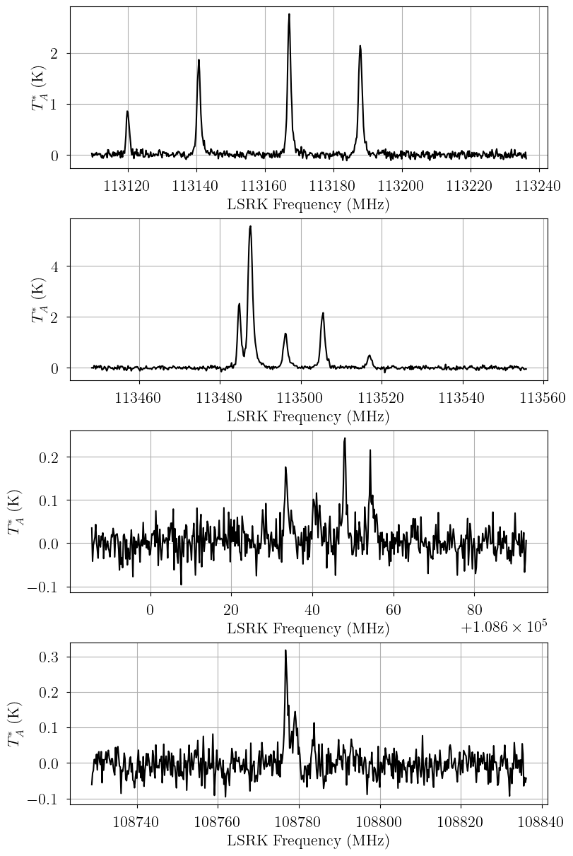
Here we test bayes_cn_hfs on some real IRAM 30-m data and demonstrate a general procedure for determining the carbon isotopic ratio from observations of CN and 13CN.

# General imports
import os
import pickle
import time

import matplotlib.pyplot as plt
import arviz as az
import pandas as pd
import numpy as np
import pymc as pm

print("arviz version:", az.__version__)

print("pymc version:", pm.__version__)

import bayes_spec
print("bayes_spec version:", bayes_spec.__version__)

import bayes_cn_hfs
print("bayes_cn_hfs version:", bayes_cn_hfs.__version__)

# Notebook configuration
pd.options.display.max_rows = None

arviz version: 0.22.0dev
pymc version: 5.21.1
bayes_spec version: 1.7.8
bayes_cn_hfs version: 2.0.0-staging+0.g7afe3a8.dirty

Load the data

from bayes_spec import SpecData
import pickle

with open("iram_data.pkl", "rb") as f:
    iram_data = pickle.load(f)

labels = ["12CN-1/2", "12CN-3/2", "13CN-1/2", "13CN-3/2"]
data = {
    label: SpecData(
        iram_data[f"frequency_{label}"][500:-500],
        iram_data[f"spectrum_{label}"][500:-500],
        iram_data[f"rms_{label}"],
        xlabel=r"LSRK Frequency (MHz)",
        ylabel=r"$T_A^*$ (K)",
    )
    for label in labels
}

# subset of 12CN data
data_12CN = {
    label: data[label]
    for label in labels if "12CN" in label
}

# Plot the data
fig, axes = plt.subplots(4, layout="constrained", figsize=(8, 12))
for i, label in enumerate(labels):
    axes[i].plot(data[label].spectral, data[label].brightness, 'k-')
    axes[i].set_xlabel(data[label].xlabel)
    axes[i].set_ylabel(data[label].ylabel)

Inspecting the CN data

We don’t assume LTE, but we fix the kinetic temperature.

from bayes_cn_hfs import CNModel

# Initialize and define the model
baseline_degree = 0
n_clouds = 2
model = CNModel(
    data_12CN,
    molecule="CN", # molecule (either "CN" or "13CN")
    bg_temp = 2.7, # assumed background temperature (K)
    Beff=0.78, # Main beam efficiency
    Feff=0.94, # Forward efficiency
    n_clouds=n_clouds,
    baseline_degree=baseline_degree,
    seed=1234,
    verbose=True
)
model.add_priors(
    prior_log10_N = [14.0, 1.0], # mean and width of log10 total column density prior (cm-2)
    prior_log10_Tkin = None, # ignored
    prior_velocity = [10.0, 3.0], # mean and width of velocity prior (km/s)
    prior_fwhm_nonthermal = 1.0, # width of non-thermal broadening prior (km/s)
    prior_fwhm_L = None, # assume Gaussian line profile
    prior_rms = None, # do not infer spectral rms
    prior_baseline_coeffs = None, # use default baseline priors
    assume_LTE = False, # do not assume LTE
    prior_log10_Tex = [0.75, 0.25], # mean and width of log10 excitation temperature prior (K)
    assume_CTEX = False, # do not assume CTEX
    prior_log10_LTE_precision = [-6.0, 1.0], # offset and width of log10 LTE precision prior
    fix_log10_Tkin = 0.5, # fix the kinetic temperature
    clip_weights = 1.0e-9, # clip statistical weights between [clip_weights, 1-clip_weights]
    clip_tau = -10.0, # clip optical depths below to prevent masers
    ordered = False, # do not assume optically-thin
)
model.add_likelihood()

from bayes_spec.plots import plot_predictive

# prior predictive check
prior = model.sample_prior_predictive(
    samples=1000,  # prior predictive samples
)
_ = plot_predictive(model.data, prior.prior_predictive)

start = time.time()
model.fit(
    n = 100_000, # maximum number of VI iterations
    draws = 1_000, # number of posterior samples
    rel_tolerance = 0.05, # VI relative convergence threshold
    abs_tolerance = 0.05, # VI absolute convergence threshold
    learning_rate = 0.01, # VI learning rate
)
end = time.time()
print(f"Runtime: {(end-start)/60.0:.2f} minutes")

posterior = model.sample_posterior_predictive(
    thin=10, # keep one in {thin} posterior samples
)
_ = plot_predictive(model.data, posterior.posterior_predictive)

pm.summary(model.trace.posterior)

start = time.time()
init_kwargs = {
    "rel_tolerance": 0.05,
    "abs_tolerance": 0.05,
    "learning_rate": 0.01,
}
model.sample(
    init = "advi+adapt_diag", # initialization strategy
    tune = 1000, # tuning samples
    draws = 1000, # posterior samples
    chains = 8, # number of independent chains
    cores = 8, # number of parallel chains
    init_kwargs = init_kwargs, # VI initialization arguments
    nuts_kwargs = {"target_accept": 0.8}, # NUTS arguments
)
end = time.time()
print(f"Runtime: {(end-start)/60.0:.2f} minutes")

model.solve(kl_div_threshold=0.1)

posterior = model.sample_posterior_predictive(
    thin=10, # keep one in {thin} posterior samples
)
_ = plot_predictive(model.data, posterior.posterior_predictive)

pm.summary(model.trace.solution_0)

Number of cloud components

from bayes_spec import Optimize
from bayes_cn_hfs import CNModel

max_n_clouds = 8
baseline_degree = 0
opt = Optimize(
    CNModel,
    data_12CN,
    molecule="CN", # molecule name
    bg_temp = 2.7, # assumed background temperature (K)
    Beff=0.78, # Main beam efficiency
    Feff=0.94, # Forward efficiency
    max_n_clouds=max_n_clouds,
    baseline_degree=baseline_degree,
    seed=1234,
    verbose=True
)
opt.add_priors(
    prior_log10_N = [14.0, 1.0], # mean and width of log10 total column density prior (cm-2)
    prior_log10_Tkin = None, # ignored
    prior_velocity = [10.0, 3.0], # mean and width of velocity prior (km/s)
    prior_fwhm_nonthermal = 1.0, # width of non-thermal broadening prior (km/s)
    prior_fwhm_L = None, # assume Gaussian line profile
    prior_rms = None, # do not infer spectral rms
    prior_baseline_coeffs = None, # use default baseline priors
    assume_LTE = False, # do not assume LTE
    prior_log10_Tex = [0.75, 0.25], # mean and width of log10 excitation temperature prior (K)
    assume_CTEX = False, # do not assume CTEX
    prior_log10_LTE_precision = [-6.0, 1.0], # offset and width of log10 LTE precision prior
    fix_log10_Tkin = 0.5, # fix the kinetic temperature
    clip_weights = 1.0e-9, # clip statistical weights between [clip_weights, 1-clip_weights]
    clip_tau = -10.0, # clip optical depths below to prevent masers
    ordered = False, # do not assume optically-thin
)
opt.add_likelihood()

from bayes_spec.plots import plot_predictive

# prior predictive check
prior = opt.models[1].sample_prior_predictive(
    samples=1000,  # prior predictive samples
)
_ = plot_predictive(opt.models[1].data, prior.prior_predictive)

start = time.time()
fit_kwargs = {
    "rel_tolerance": 0.05,
    "abs_tolerance": 0.05,
    "learning_rate": 0.01,
}
opt.fit_all(**fit_kwargs)
end = time.time()
print(f"Runtime: {(end-start)/60.0:.2f} minutes")

null_bic = opt.models[1].null_bic()
n_clouds = np.arange(max_n_clouds+1)
bics_vi = np.array([null_bic] + [model.bic(chain=0) for model in opt.models.values()])
print(bics_vi)

plt.plot(n_clouds[1:], bics_vi[1:], 'ko')

start = time.time()
fit_kwargs = {
    "rel_tolerance": 0.05,
    "abs_tolerance": 0.05,
    "learning_rate": 0.01,
}
sample_kwargs = {
    "chains": 8,
    "cores": 8,
    "n_init": 100_000,
    "init_kwargs": fit_kwargs,
    "nuts_kwargs": {"target_accept": 0.9},
}
opt.optimize(fit_kwargs=fit_kwargs, sample_kwargs=sample_kwargs, approx=False)
end = time.time()
print(f"Runtime: {(end-start)/60.0:.2f} minutes")

null_bic = opt.models[1].null_bic()
n_clouds = np.arange(max_n_clouds+1)
bics_mcmc = np.array([null_bic] + [model.bic() for model in opt.models.values()])
print(bics_mcmc)

plt.plot(n_clouds[1:], bics_vi[1:], 'ko', label="VI")
plt.plot(n_clouds[1:], bics_mcmc[1:], 'ro', label="MCMC")
plt.xlabel("Number of Clouds")
plt.ylabel("BIC")
_ = plt.legend()

model = opt.models[2]
print(model.n_clouds)
pm.summary(model.trace.solution_0)

posterior = model.sample_posterior_predictive(
    thin=100, # keep one in {thin} posterior samples
)
_ = plot_predictive(model.data, posterior.posterior_predictive)

Ratio Model

We start by assuming CTEX for 13CN.

from bayes_cn_hfs.cn_ratio_model import CNRatioModel

# Initialize and define the model
n_clouds = 2 # number of cloud components
baseline_degree = 0 # polynomial baseline degree
model = CNRatioModel(
    data,
    bg_temp = 2.7, # assumed background temperature (K)
    Beff=0.78, # Main beam efficiency
    Feff=0.94, # Forward efficiency
    n_clouds=n_clouds,
    baseline_degree=baseline_degree,
    seed=1234,
    verbose=True
)
model.add_priors(
    prior_log10_N_12CN = [14.5, 0.5], # mean and width of log10 12CN total column density prior (cm-2)
    prior_ratio_12C_13C = [50.0, 25.0], # mean and width of 12C/13C ratio prior
    prior_log10_Tkin = None, # kinetic temperature is fixed
    prior_velocity = [9.0, 2.0], # mean and width of velocity prior (km/s)
    prior_fwhm_nonthermal = 1.0, # width of non-thermal broadening prior (km/s)
    prior_fwhm_L = 1.0, # width of latent Lorentzian FWHM prior (km/s) TIP: set to typical feature separation
    prior_rms = None, # do not infer spectral rms
    prior_baseline_coeffs = None, # use default baseline priors
    assume_LTE = False, # do not assume LTE
    prior_log10_Tex = [0.6, 0.15], # mean and width of excitation temperature prior (K)
    assume_CTEX_12CN = False, # do not assume CTEX
    prior_LTE_precision = 100.0, # width of LTE precision prior
    assume_CTEX_13CN = True, # assume CTEX for 13CN
    fix_log10_Tkin = 1.5, # kinetic temperature is fixed (K)
    ordered = False, # do not assume optically-thin
)
model.add_likelihood()

from bayes_spec.plots import plot_predictive

# prior predictive check
prior = model.sample_prior_predictive(
    samples=100,  # prior predictive samples
)
_ = plot_predictive(model.data, prior.prior_predictive)

start = time.time()
model.fit(
    n = 100_000, # maximum number of VI iterations
    draws = 1_000, # number of posterior samples
    rel_tolerance = 0.01, # VI relative convergence threshold
    abs_tolerance = 0.1, # VI absolute convergence threshold
    learning_rate = 0.01, # VI learning rate
)
end = time.time()
print(f"Runtime: {(end-start)/60.0:.2f} minutes")

posterior = model.sample_posterior_predictive(
    thin=100, # keep one in {thin} posterior samples
)
_ = plot_predictive(model.data, posterior.posterior_predictive)

start = time.time()
model.sample(
    init = "advi+adapt_diag", # initialization strategy
    tune = 1000, # tuning samples
    draws = 1000, # posterior samples
    chains = 8, # number of independent chains
    cores = 8, # number of parallel chains
    init_kwargs = {"rel_tolerance": 0.01, "abs_tolerance": 0.1, "learning_rate": 0.01}, # VI initialization arguments
    nuts_kwargs = {"target_accept": 0.9}, # NUTS arguments
)
end = time.time()
print(f"Runtime: {(end-start)/60.0:.2f} minutes")

model.solve(kl_div_threshold=0.1)

print("solutions:", model.solutions)

pm.summary(model.trace.solution_0)

posterior = model.sample_posterior_predictive(
    thin=100, # keep one in {thin} posterior samples
)
_ = plot_predictive(model.data, posterior.posterior_predictive)

# 12C/13C ratio over all clouds
for solution in model.solutions:
    model.trace[f"solution_{solution}"]["ratio_12C_13C_total"] = (
        (10.0**model.trace[f"solution_{solution}"]["log10_N_12CN"]).sum(dim="cloud") /
    model.trace[f"solution_{solution}"]["N_13CN"].sum(dim="cloud")
    )

pm.summary(model.trace.solution_0, var_names=["ratio_12C_13C_total"])

import pickle
with open("/staging/twenger2/iram_trace.pkl", "wb") as f:
    pickle.dump(model.trace, f)

from bayes_spec.plots import plot_pair

var_names = [
    param for param in model.cloud_freeRVs
    if not set(model.model.named_vars_to_dims[param]).intersection(set(
        ["transition_12CN", "state_12CN", "transition_13CN", "state_13CN"]
    ))
]
_ = plot_pair(
    model.trace.solution_0, # samples
    var_names, # var_names to plot
    labeller=model.labeller, # label manager
)

# ignore transition and state dependent parameters
var_names = [
    param for param in model.cloud_deterministics + ["ratio_12C_13C"]
    if not set(model.model.named_vars_to_dims[param]).intersection(set(
        ["transition_12CN", "state_12CN", "transition_13CN", "state_13CN"]
    )) and param not in ["fwhm_thermal_12CN", "fwhm_thermal_13CN"]
]
print(var_names)
_ = plot_pair(
    model.trace.solution_0.sel(cloud=0), # samples
    var_names + model.hyper_deterministics, # var_names to plot
    labeller=model.labeller, # label manager
)

_ = plot_pair(
    model.trace.solution_0.sel(cloud=1), # samples
    var_names + model.hyper_deterministics, # var_names to plot
    labeller=model.labeller, # label manager
)

var_names = model.cloud_deterministics + model.baseline_freeRVs + model.hyper_freeRVs + model.hyper_deterministics + ["ratio_12C_13C", "ratio_12C_13C_total"]
point_stats = az.summary(model.trace.solution_0, var_names=var_names, kind='stats', hdi_prob=0.68)
display(point_stats)

Assumption about 13CN Excitation Temperature

There is no evidence for CTEX in the 13CN data, and we are unable to constrain the excitation temperature of 13CN because we only detect the brightest transitions. Here we relax the 13CN CTEX assumption and instead assume that it suffers from hyperfine anomalies the same as 12CN.

from bayes_cn_hfs.cn_ratio_model import CNRatioModel

# Initialize and define the model
n_clouds = 2 # number of cloud components
baseline_degree = 0 # polynomial baseline degree
model = CNRatioModel(
    data,
    bg_temp = 2.7, # assumed background temperature (K)
    Beff=0.78, # Main beam efficiency
    Feff=0.94, # Forward efficiency
    n_clouds=n_clouds,
    baseline_degree=baseline_degree,
    seed=1234,
    verbose=True
)
model.add_priors(
    prior_log10_N_12CN = [14.5, 0.5], # mean and width of log10 12CN total column density prior (cm-2)
    prior_ratio_12C_13C = [50.0, 25.0], # mean and width of 12C/13C ratio prior
    prior_log10_Tkin = None, # kinetic temperature is fixed
    prior_velocity = [9.0, 2.0], # mean and width of velocity prior (km/s)
    prior_fwhm_nonthermal = 1.0, # width of non-thermal broadening prior (km/s)
    prior_fwhm_L = 1.0, # width of latent Lorentzian FWHM prior (km/s) TIP: set to typical feature separation
    prior_rms = None, # do not infer spectral rms
    prior_baseline_coeffs = None, # use default baseline priors
    assume_LTE = False, # do not assume LTE
    prior_log10_Tex = [0.6, 0.15], # mean and width of excitation temperature prior (K)
    assume_CTEX_12CN = False, # do not assume CTEX
    prior_LTE_precision = 100.0, # width of LTE precision prior
    assume_CTEX_13CN = False, # assume CTEX for 13CN
    fix_log10_Tkin = 1.5, # kinetic temperature is fixed (K)
    ordered = False, # do not assume optically-thin
)
model.add_likelihood()

from bayes_spec.plots import plot_predictive

# prior predictive check
prior = model.sample_prior_predictive(
    samples=100,  # prior predictive samples
)
_ = plot_predictive(model.data, prior.prior_predictive)

start = time.time()
model.fit(
    n = 100_000, # maximum number of VI iterations
    draws = 1_000, # number of posterior samples
    rel_tolerance = 0.01, # VI relative convergence threshold
    abs_tolerance = 0.1, # VI absolute convergence threshold
    learning_rate = 0.01, # VI learning rate
)
end = time.time()
print(f"Runtime: {(end-start)/60.0:.2f} minutes")

posterior = model.sample_posterior_predictive(
    thin=100, # keep one in {thin} posterior samples
)
_ = plot_predictive(model.data, posterior.posterior_predictive)

start = time.time()
model.sample(
    init = "advi+adapt_diag", # initialization strategy
    tune = 1000, # tuning samples
    draws = 1000, # posterior samples
    chains = 8, # number of independent chains
    cores = 8, # number of parallel chains
    init_kwargs = {"rel_tolerance": 0.01, "abs_tolerance": 0.1, "learning_rate": 0.01}, # VI initialization arguments
    nuts_kwargs = {"target_accept": 0.9}, # NUTS arguments
)
end = time.time()
print(f"Runtime: {(end-start)/60.0:.2f} minutes")

model.solve(kl_div_threshold=0.1)

print("solutions:", model.solutions)

pm.summary(model.trace.solution_0)

posterior = model.sample_posterior_predictive(
    thin=100, # keep one in {thin} posterior samples
)
_ = plot_predictive(model.data, posterior.posterior_predictive)

# 12C/13C ratio over all clouds
for solution in model.solutions:
    model.trace[f"solution_{solution}"]["ratio_12C_13C_total"] = (
        (10.0**model.trace[f"solution_{solution}"]["log10_N_12CN"]).sum(dim="cloud") /
    model.trace[f"solution_{solution}"]["N_13CN"].sum(dim="cloud")
    )

pm.summary(model.trace.solution_0, var_names=["ratio_12C_13C_total"])

import pickle
with open("/staging/twenger2/iram_trace_noCTEX.pkl", "wb") as f:
    pickle.dump(model.trace, f)